MEA: Step-wise Analysis: Example

In this example code, we demonstrate analysis of MEA Recording, with each step. There are 13 steps.

1. Read HDF File

2. Stim loc

3. Align Cycles

4. Average Cycles/Select one

5. Activation Time

6. Activation & Repolarisation Time

7. APD computation

8. Extract EGM

9. EGM Feature Extraction

10. BAD Channels

11. Feature Matrix

12. Interpolation

13. Conduction Velocity

#sp.mea
import numpy as np
import matplotlib.pyplot as plt
import os, requests
import spkit as sp
print('spkit-version: ',sp.__version__)

# Download Sample file if not done already

file_name= 'MEA_Sample_North_1000mV_1Hz.h5'

if not(os.path.exists(file_name)):
    path = 'https://spkit.github.io/data_samples/files/MEA_Sample_North_1000mV_1Hz.h5'
    req = requests.get(path)
    with open(file_name, 'wb') as f:
            f.write(req.content)

spkit-version:  0.0.9.7

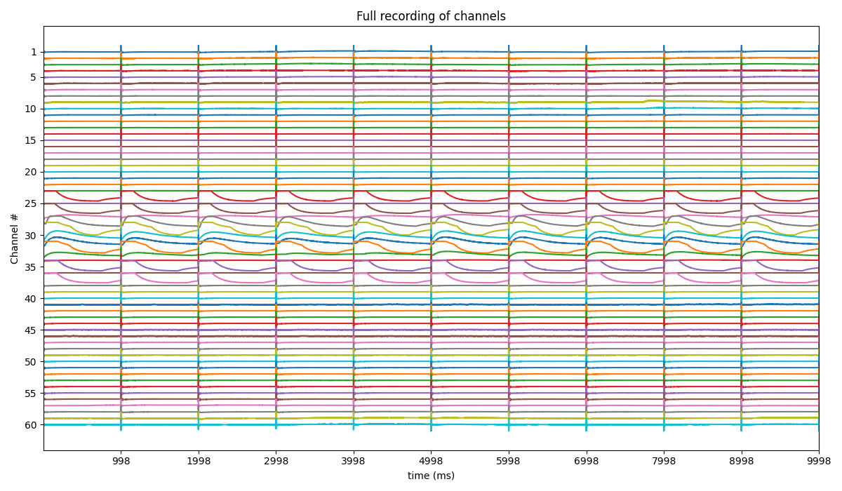
Step 1: Read File

fs = 25000
X,fs,ch_labels = sp.io.read_hdf(file_name,fs=fs,verbose=1)

base key(s) found in file <KeysViewHDF5 ['Data']>
Shape of Signals:  (60, 250000)
- #Channels    = 60
- Duration (s) = 10.0

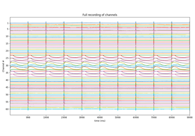
Step 2: Stim Localisation

stim_fhz = 1
stim_loc,_  = sp.mea.get_stim_loc(X,fs=fs,fhz=stim_fhz, plot=1,verbose=1)

stim_loc_ms = 1000*np.array(stim_loc)/fs


t = 1000*np.arange(X.shape[1])/fs
sep = 1000
tix = np.arange(len(X))*sep
tiy = np.arange(0,len(X)+1,5)
tiy[0] =1
plt.figure(figsize=(12,7))
plt.plot(t,X.T - tix)
plt.xlim([t[0],t[-1]])
plt.yticks(-(tiy-1)*sep,tiy,fontsize=10)
plt.ylabel('Channel #')
plt.xlabel('time (ms)')
plt.title('Full recording of channels')
plt.xticks(stim_loc_ms)
plt.tight_layout()
plt.show()

• 
• 

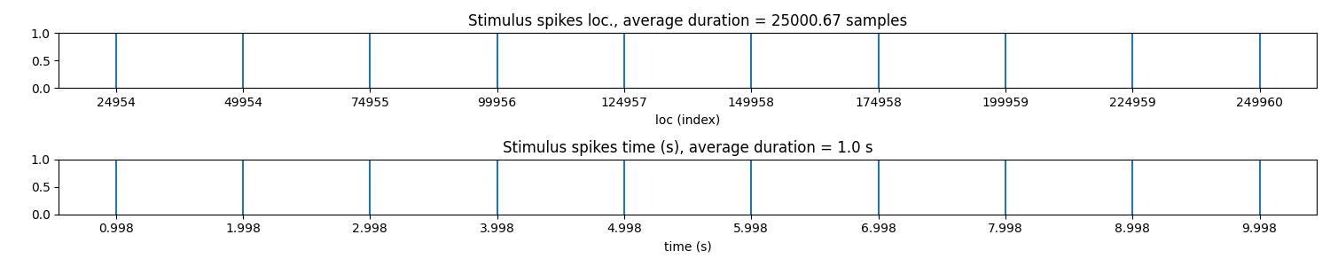
-#cycles= 10

Step 3: Align Cycles

exclude_first_dur=2
dur_after_spike=500
exclude_last_cycle=True

XB = sp.mea.align_cycles(X,stim_loc,fs=fs, exclude_first_dur=exclude_first_dur,dur_after_spike=dur_after_spike,
                         exclude_last_cycle=exclude_last_cycle,pad=np.nan,verbose=True)

print('Number of EGMs/Cycles per channel =',XB.shape[2])
ch = 0
t = 1000*np.arange(XB.shape[1])/fs
plt.figure(figsize=(5,4))
plt.plot(t,XB[ch,:,:])
plt.grid()
plt.title(f'{XB.shape[2]} Cycles (Alinged) of Channel: {ch}')
plt.xlabel('time (ms)')
plt.show()

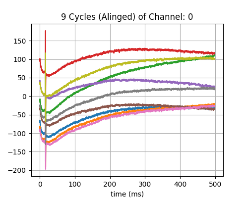
Shape: (60, 12450, 9)
Number of EGMs/Cycles per channel = 9

Step 4: Average Cycles or Select one

egm_number = -1

if egm_number<0:
    X1B = np.nanmean(XB,axis=2)
    print(' -- Averaged All EGM')
else:
    # egm_number should be between from 0 to 'Number of EGMs/Cycles per channel '
    assert egm_number in list(range(XB.shape[2]))
    X1B = XB[:,:,egm_number]
    print(' -- Selected EGM ->',egm_number)

print('EGM Shape : ',X1B.shape)

 -- Averaged All EGM
EGM Shape :  (60, 12450)

Step 5-6: Activation and Repolarisation Time

#at_range = [0,100]
#rt_range = [2,100]
at_range=[0,None]
rt_range= [0.5, None]

# for only activation
at_loc = sp.mea.activation_time_loc(X1B,fs=fs,at_range=at_range)

# for only activation and repolarisation together
at_loc, rt_loc = sp.mea.activation_repol_time_loc(X1B,fs=fs,at_range=at_range, rt_range=rt_range)

at_loc_ms = 1000*at_loc/fs
rt_loc_ms = 1000*rt_loc/fs

at_loc_ms, rt_loc_ms

(array([ 16.64,  19.56,  13.96,  10.88,  19.52,  16.88,  20.04,  14.04,
       323.44,  18.6 ,  14.84,  16.16,  11.48,  12.4 , 284.08,  10.64,
         9.48,   8.24,   9.  ,   7.  ,   8.04,   5.  ,   5.48, 174.48,
         2.72, 176.4 ,   8.04, 357.  , 394.88,   1.84, 349.76, 345.48,
         4.72,   7.88, 209.08,   1.48, 201.6 ,   4.64,   2.68,   4.12,
       330.32,   6.56,   7.56,   7.92,   9.24, 343.92,  10.96,  10.52,
        14.32,  13.76,  17.12,  16.68,  13.6 ,  19.68,  16.48,  19.48,
        11.16,  13.92,  19.52,  16.76]), array([349.76, 323.4 , 278.08,  44.6 , 472.64, 120.6 , 424.96, 472.64,
       340.32, 302.92, 271.48, 472.64,  16.16,  16.16, 314.8 ,  11.36,
        10.68,   9.52,  12.04,   9.12,  44.6 , 429.52, 407.48, 202.68,
       342.48, 201.6 , 351.84, 357.96, 419.36, 425.  , 351.88, 351.84,
       316.36, 460.  , 219.32, 278.08, 235.56, 295.76, 323.4 , 323.4 ,
       343.92, 349.76, 342.48, 202.68, 330.28, 357.04, 351.84, 145.2 ,
       245.88, 472.64, 278.08, 323.4 , 397.28, 295.76, 349.76, 349.76,
        44.6 ,  44.6 ,  83.16,  93.72]))

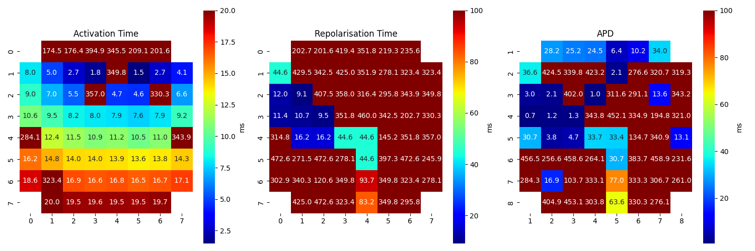
Step 7: APD Computation

apd_ms = rt_loc_ms-at_loc_ms

AT_grid = sp.mea.arrange_mea_grid(at_loc_ms, ch_labels=ch_labels)
RT_grid = sp.mea.arrange_mea_grid(rt_loc_ms, ch_labels=ch_labels)
APD_grid = sp.mea.arrange_mea_grid(apd_ms, ch_labels=ch_labels)

fig, ax = plt.subplots(1,3, figsize=(15,5))
sp.mea.mat_1_show(AT_grid,vmax=20, label = ('ms'),ax=ax[0])
ax[0].set_title('Activation Time')
sp.mea.mat_1_show(RT_grid,vmax=100,label = ('ms'),ax=ax[1])
ax[1].set_title('Repolarisation Time')
sp.mea.mat_1_show(APD_grid,vmax=100, label = ('ms'),ax=ax[2])
ax[2].set_title('APD')
plt.tight_layout()
plt.show()

Step 8: Extract EGMs

dur_from_loc = 5
remove_drift = True

XE,ATloc = sp.mea.extract_egm(X1B,act_loc=at_loc,fs=fs,dur_from_loc=dur_from_loc,remove_drift=remove_drift)
print(XE.shape, ATloc.shape)

(60, 250) (60,)

Step 9: EGM Feature Extraction

EGM_feat = []
for i in range(len(XE)):
    egmf, feat_names = sp.mea.egm_features(XE[i].copy(),act_loc=ATloc[i],fs=fs,plot=0,verbose=0,width_rel_height=0.75,
                                   findex_rel_dur=1, findex_rel_height=0.3, findex_npeak=False)
    EGM_feat.append(egmf)

#XE = np.array(XE)
#ATloc = np.array(ATloc)
EGM_feat = np.array(EGM_feat)

print('-'*100)
print('Following EGM Features are etracted: ', feat_names)
print('EGM_Feat shape :',EGM_feat.shape)
print('Shapes: XE =',XE.shape, ', AT =',ATloc.shape,', EGM_F=' ,EGM_feat.shape)
print('-'*100)

----------------------------------------------------------------------------------------------------
Following EGM Features are etracted:  ['peak_to_peak', 'egm_duration', 'f_index', 'new_duration', 'energy_mean', 'energy_sd', 'noise_var']
EGM_Feat shape : (60, 7)
Shapes: XE = (60, 250) , AT = (60,) , EGM_F= (60, 7)
----------------------------------------------------------------------------------------------------

Step 10: BAD Channels

#=============STEP 10.1: BAD Channel (1) ================================
good_channels = []
bad_channels = [15]

p2p_thr=5
bad_ch_stim_thr = 2
bad_ch_mnmx=[None, None]

range_act_thr=[0,50]

bad_channels_list =[]
bad_channels_idx_1 = []

bad_channels_idx_1 = sp.mea.find_bad_channels_idx(X,thr=bad_ch_stim_thr,stim_fhz=stim_fhz,fs=fs,
                    mnmx=bad_ch_mnmx,plot=False,plot_dur=2,verbose=0)
bad_channels_ch_1  = list(ch_labels[bad_channels_idx_1])
bad_channels_list  = bad_channels_list + bad_channels_ch_1
bad_channels_list  = list(set(bad_channels_list))
bad_channels_list.sort()

#=============STEP 10.2: BAD Channel (2) ================================
bad_channels_idx_2 = []
bad_channels_idx_2 = np.where(EGM_feat[:,0]<p2p_thr)[0]
bad_channels_ch_2 = list(ch_labels[bad_channels_idx_2])
bad_channels_list = bad_channels_list + bad_channels_ch_2


#=============STEP 10.3: BAD Channel (3) ================================
bad_channels_idx_3 =[]
bad_channels_idx_3 = bad_channels_idx_3 + list(np.where(at_loc_ms<range_act_thr[0])[0])
bad_channels_idx_3 = bad_channels_idx_3 + list(np.where(at_loc_ms>range_act_thr[1])[0])
bad_channels_ch_3 = list(ch_labels[bad_channels_idx_3])
bad_channels_list = bad_channels_list + bad_channels_ch_3

bad_channels_list = bad_channels_list + bad_channels
bad_channels_list = list(set(bad_channels_list))
bad_channels_list.sort()

if len(good_channels):
    bad_channels_list = list(set(bad_channels_list) - set(good_channels))
    bad_channels_list.sort()


good_channels_list = np.array([ch for ch in ch_labels if ch not in bad_channels_list])
good_channels_list_idx = np.array([list(ch_labels).index(ch) for ch in ch_labels if ch not in bad_channels_list])

print('-'*100)
print('BAD CHANNELS')
print('- BASED ON STIM thr =', bad_ch_stim_thr)
print('  - ch:', bad_channels_ch_1)
print('- BASED ON Peak-to-Peak volt thr:',p2p_thr)
print('  - ch:', bad_channels_ch_2)
print('- BASED ON Activation time (ms) range thr:', range_act_thr)
print('  - ch:', bad_channels_ch_3)
print('- Manually passed:')
print('  - ch:', bad_channels)
print('GOOD CHANNELS passed:')
print('  - ch:',good_channels)
print('-'*50)
print('Final list of Bad Channels:')
print(' - ch:',bad_channels_list)
print('Final list of Good Channels:')
print(' - ch:',good_channels_list)
print('-'*100)


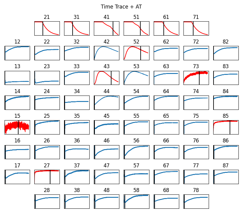
sp.mea.plot_mea_grid(X1B,act_spikes=at_loc,ch_labels=ch_labels,bad_channels=bad_channels_list,
                     xlim=at_range,verbose=True,
                     figsize=(8,7),title_style=1, title='Time Trace + AT')

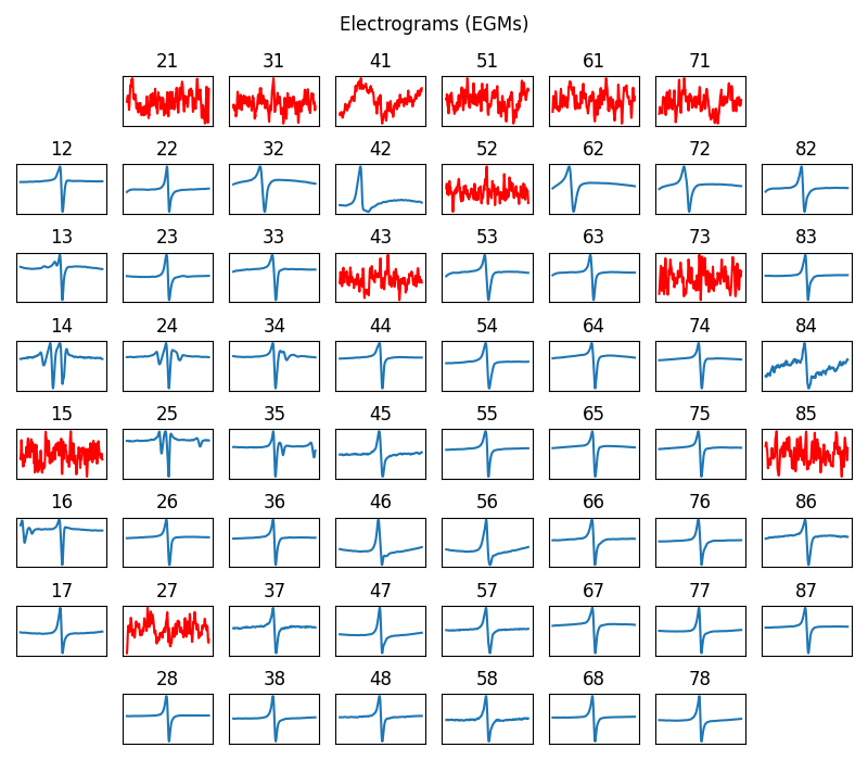
sp.mea.plot_mea_grid(XE,ch_labels=ch_labels,bad_channels=bad_channels_list,
                     figsize=(8,7),verbose=0,show=True,title_style=1,title='Electrograms (EGMs)')

• 
• 

----------------------------------------------------------------------------------------------------
BAD CHANNELS
- BASED ON STIM thr = 2
  - ch: [21, 31, 43, 41, 51, 61, 71]
- BASED ON Peak-to-Peak volt thr: 5
  - ch: [15, 21, 31, 43, 41, 52, 51, 61, 71]
- BASED ON Activation time (ms) range thr: [0, 50]
  - ch: [27, 15, 21, 31, 43, 41, 52, 51, 61, 71, 73, 85]
- Manually passed:
  - ch: [15]
GOOD CHANNELS passed:
  - ch: []
--------------------------------------------------
Final list of Bad Channels:
 - ch: [15, 21, 27, 31, 41, 43, 51, 52, 61, 71, 73, 85]
Final list of Good Channels:
 - ch: [47 48 46 45 38 37 28 36 17 26 16 35 25 14 24 34 13 23 12 22 33 32 44 42
 53 54 62 63 72 82 83 64 74 84 75 65 86 76 87 77 66 78 67 68 55 56 58 57]
----------------------------------------------------------------------------------------------------
-852.8768781599376 1088.2322322933303

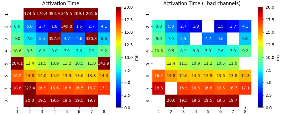
Step 11: Feature Matrix

Ax,Mxbad = sp.mea.mea_feature_map(at_loc_ms,ch_labels=ch_labels,bad_channels=bad_channels_list,figsize=(10,4),
                               vmin=0,vmax=20,label='ms',title='Activation Time')

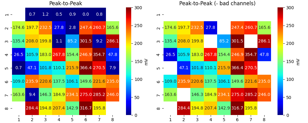
_ = sp.mea.mea_feature_map(EGM_feat[:,0],ch_labels=ch_labels,bad_channels=bad_channels_list,figsize=(10,4),
                               vmin=0,vmax=300,label='mV',title='Peak-to-Peak')


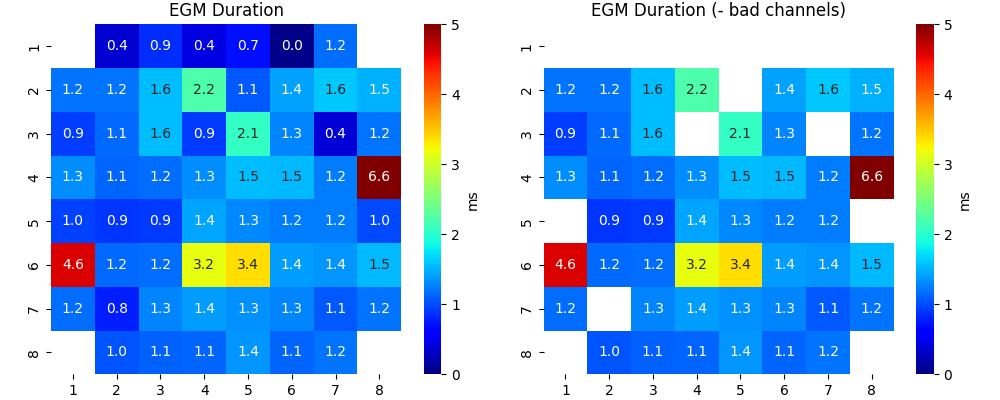
_ = sp.mea.mea_feature_map(1000*EGM_feat[:,1]/fs,ch_labels=ch_labels,bad_channels=bad_channels_list,figsize=(10,4),
                               vmin=0,vmax=5,label='ms',title='EGM Duration')

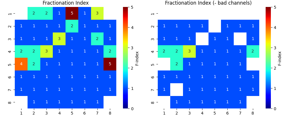
_ = sp.mea.mea_feature_map(EGM_feat[:,2],ch_labels=ch_labels,bad_channels=bad_channels_list,figsize=(10,4),
                               vmin=0,vmax=5,label='F-index',title='Fractionation Index',fmt='.0f')

• 
• 
• 
• 

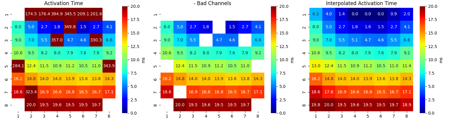
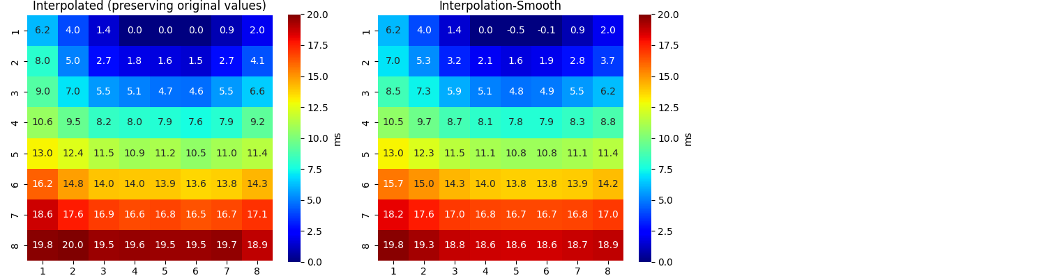
Step 12: Interpolating Activation Map

range_act_thr=[0,50]
intp_param = dict(pkind='linear',filter_size=3,method='conv')

AxI, AxIx = sp.fill_nans_2d(Ax*Mxbad,clip_range=range_act_thr,**intp_param)




sp.mea.mat_list_show([Ax, Ax*Mxbad, AxI],figsize=(15,4),vmin=0,vmax=20,grid=(1,3),
              titles=['Activation Time', '- Bad Channels', 'Interpolated Activation Time'],labels=['ms','ms','ms'])

sp.mea.mat_list_show([AxI, AxIx],figsize=(15,4),vmin=0,vmax=20,grid=(1,3),
              titles=['Interpolated (preserving original values)', 'Interpolation-Smooth'],labels=['ms','ms'])

• 
• 

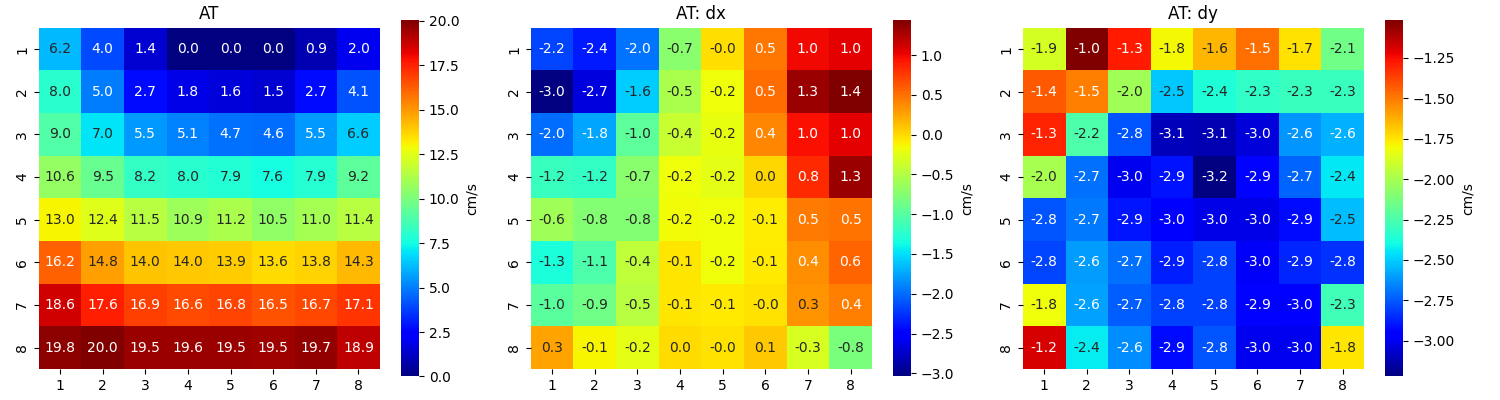
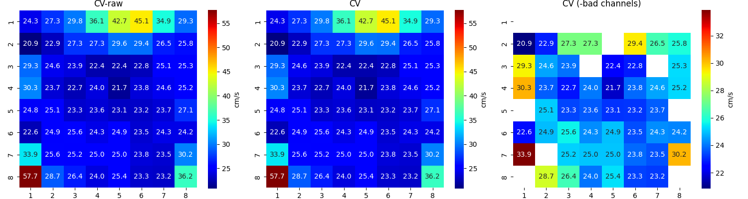
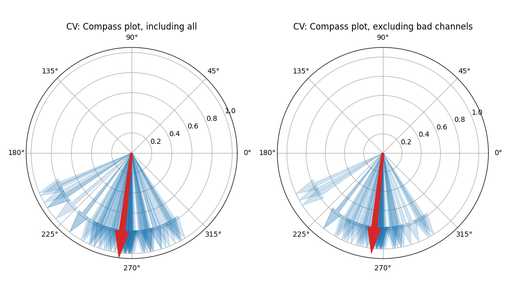
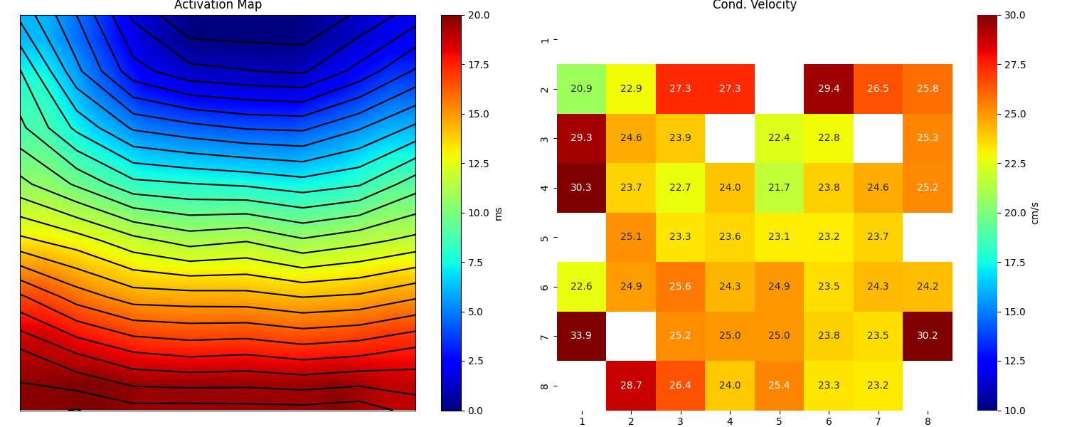
Step 13: Computing Conduction Velocity and maps

#=============STEP 13: Computing Conduction Velocity ================
cv_param = dict(eD=700,esp=1e-10,cv_pad=np.nan,cv_thr=100,arr_agg='mean',plots=2,verbose=True)

CV_df, CV_thetas, CV0, CV = sp.mea.compute_cv(AxI,Mxbad,flip=False,**cv_param)

_, CV_thetas_smooth, _, _ = sp.mea.compute_cv(AxIx,Mxbad,flip=False,silent_mode=True,**cv_param)



plt.figure(figsize=(15,6))
plt.subplot(121)
im = plt.imshow(AxI,cmap='jet',interpolation='bilinear',vmin=0,vmax=20,extent=[0,7,7,0])
plt.contour(AxI,levels=25,colors='k')
plt.colorbar(im, label='ms')
plt.title('Activation Map')
plt.xticks([])
plt.yticks([])
plt.subplot(122)
sp.mea.mat_1_show(CV*Mxbad,fmt='.1f',vmin=10,vmax=30,cmap='jet',label='cm/s',title='Cond. Velocity')
plt.tight_layout()
plt.show()

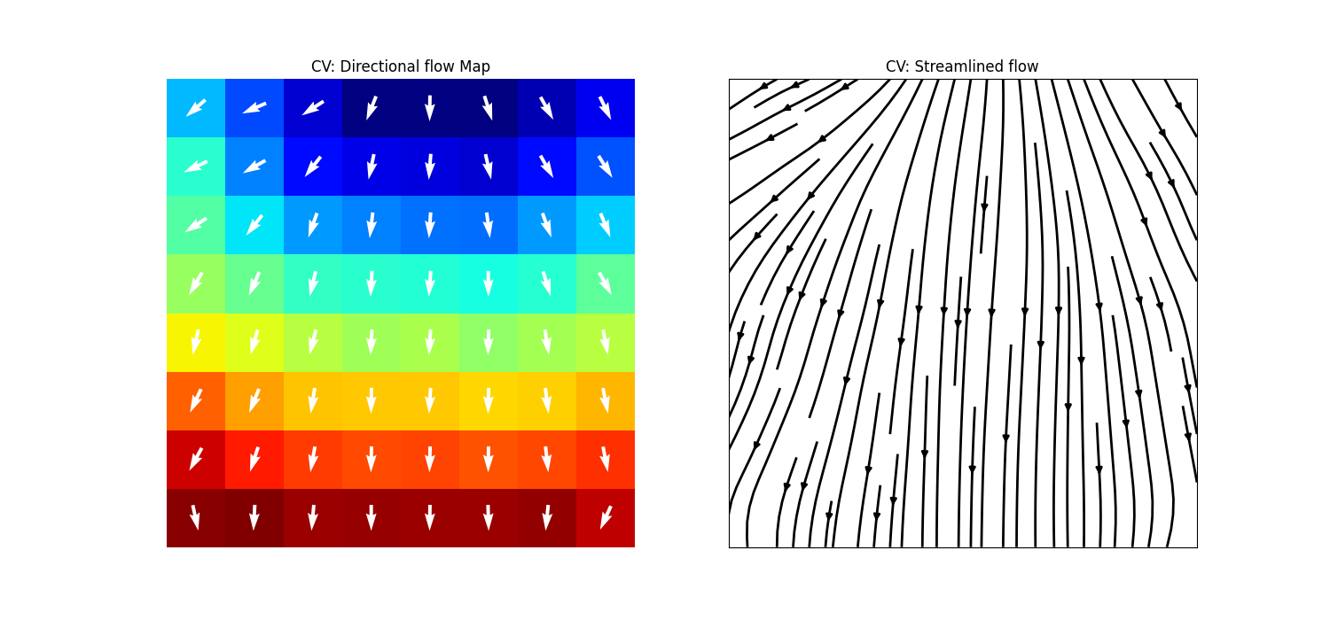
cv_arr_prop = dict(color='w',scale=None)

_  = sp.direction_flow_map(X_theta=CV_thetas,X=AxI,upsample=1,
                            figsize=(15,7),square=True,cbar=False,arr_pivot='mid',
                           stream_plot=True,title='CV',show=True,
                           heatmap_prop =dict(vmin=0,vmax=20,cmap='jet'),
                           arr_prop =cv_arr_prop,
                           stream_prop =dict(density=1,color='k',linewidth=2))

• 
• 
• 
• 
• 
• 

Related examples

MEA: Minimal Setting: Example

MEA: Minimal Setting: Example

EEG Data from EDF File

EEG Data from EDF File

ATAR Algorithm with MNE RAW Object

ATAR Algorithm with MNE RAW Object

Dispersion Entropy with top patterns

Dispersion Entropy with top patterns

EEG Artifact removal using ICA

EEG Artifact removal using ICA