spkit.mea.egm_features
- spkit.mea.egm_features(x, act_loc, fs=25000, width_rel_height=0.75, findex_rel_dur=1, findex_rel_height=0.75, findex_npeak=False, verbose=1, plot=1, figsize=(8, 3), title='', **kwargs)
Feature Extraction from a single EGM
Feature Extraction from a single EGM
Following features are extracted from given EGM x
Peak to Peak voltage
Duration of EGM
Fractional Index
Refined Duration of EGM based on fractionating peaks
Energy of EGM
Voltage Dispersion
Noise variance
1. Peak to Peak voltage
As activation time loc is a location of maximum negative deflection, that entails a high positive peak (p1) just before activation loc followed by very low negative peak (p2) after loc. So Peak to Peak voltage is computed as volatege difference between p1 and p2. As shows pictorially
              +ve peak = v1
               |
               |  -
               |    -          p2
            ---|-------|-------|
               p1     loc      |
                          -    |
                             - |
                             -ve peak = v2

Peak to Peak voltage = |v1-v2|
2. Duration of EGM
Each peak has a width, which computed by ‘width_rel_height’
- width_rel_heightdefault=0.75
Relative hight of peaks to estimate the width of peaks,
Lower it is smaller the width of peak be, which leads to smaller duration of EGM
In this diagram, peak p1 has a width of p12-p11, where p11 is the left end of positive peak, Similarly, peak p2 has right end point of width as p22. So duration of EGM is computed as difference start of +ve peak width to end of -ve peak width, which is
duration = p22-p11

            ---!---p1---|-- | ----|---p2----!-
              p11       p12 |    p21       p22
                            |
                            |
                           loc
3. Fractionation Index
Fractionation Index is defined as number of peaks after loc (activation time), within a search region, that exceeds the threshold of height. Threshold of height defined by findex_rel_height (= findex_rel_height*positive_peak_height, findex_rel_height*negative_peak_height).
Fractionating peaks can be positive or/negative. In ideal situation, every positive peak is followed by negative one, so they come in pair. Therefore:
Fractionation Index = 1 + max(positive_fr_peaks, negative_fr_peaks)
- So:
Fractionation Index = 1, means, no extra peaks within duration, other than main peaks
Fractionation Index = 2, means, there is one peak after loc, that exceeds the threshold.
However, postive frationating peaks are more reliable and negative peaks are often due to noise. Therefore, setting findex_npeak=False, avoid consideration of negative peaks
Search Region of fractionation index is set by ‘findex_rel_dur’
- findex_rel_dur: default = 1
Relative duration of search region, to find fractionating peaks.
As explained above for duration,
duration = p22-p11

            ---|----------| -----------|-
            p11       loc          p22

Search region  = p22 +  findex_rel_dur*duration
if findex_rel_dur = 0, means searching for fractionating peaks between activation time (loc) to end point of EGM’s duration (p22)
Threshold of height defined by findex_rel_height
- findex_rel_height: default=0.75
Relative height threshold for defining the fractionation,
Any positive peak which exceeds the hight of 0.75*positive peak of EGM at loc, within Search region is considered fractionating peak
Similarly, any negative peak which goes below 0.75*negative peak of EGM at loc, within Search region is considered fractionating peak
- findex_npeak: default=False
if true, negative peaks are considered for fractionation,
4. Refined Duration
Refined Duration of EGM based on fractionating peaks
This is defined by new end point (right) of negative peak, which is the end point of last fractionating peak
5. Energy of EGM
Mean(x**2) (mean squared voltage)
6. Voltage Dispersion
SD(x**2) (SD of squared voltage)
7. Noise variance
Median(|x|)/0.6745 (Estimated noise variance)
- Parameters:
- x1d-array,
input signal (EGM)
- fsint
sampling frequency,
- act_locint,
activation time location of EGM index
- width_rel_height: scalar, default=0.75
Relative hight of peaks to estimate the width of peaks,
Lower it is smaller the width of peak be, which leads to smaller duration of EGM
- findex_rel_dur: +ve scalar, default = 1
Relative duration of search region, to find fractionating peaks.
As explained above for duration,
- findex_rel_height: scalar, default=0.75
Relative height threshold for defining the fractionation,
Any positive peak which exceeds the hight of 0.75*positive peak of EGM at loc, within Search region is considered fractionating peak
Similarly, any negative peak which goes below 0.75*negative peak of EGM at loc, within Search region is considered fractionating peak
- findex_npeak: bool, deafult=False
if true, negative peaks are considered for fractionation, default=False
- plot: if True,
plot EGM with all the features shown
- figsize=(8,3): size of figure
- verbose: 0 Silent
1 a few details 2 all the computations
- Returns:
- features: list of 7 featur values
- peak2peak: float
peak to peak voltage, with same unite as input x
- duration:float
duration of EGM in samples, output would be a float, as width of peak is computed by interpolated.
Divide it by fs to compute in seconds
duration in (s) = duration/fs
- findex: int,
Fractionation Index, number of peaks after activation that crosses the ‘findex_rel_height’ of the main peak
- new_duration: float,
New duration, refined by fractionating peaks, same in samples.
Divide it by fs to compute in seconds
- energy_mean: float,
Energy of EGM (mean squared voltage)
- energy_sd: float,
Voltage Dispersion (SD of squared voltage)
- noise_var: float,
Estimated noise variance (= median(|x|)/0.6745)
- names: list of names of each feature
See also
Examples
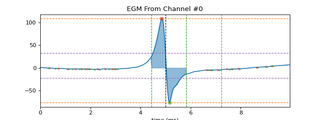
>>> #sp.mea.extract_egm
>>> import numpy as np
>>> import matplotlib.pyplot as plt
>>> import os, requests
>>> import spkit as sp
>>> # Download Sample file if not done already
>>> file_name= 'MEA_Sample_North_1000mV_1Hz.h5'
>>> if not(os.path.exists(file_name)):
>>>     path = 'https://spkit.github.io/data_samples/files/MEA_Sample_North_1000mV_1Hz.h5'
>>>     req = requests.get(path)
>>>     with open(file_name, 'wb') as f:
>>>             f.write(req.content)
>>> ##############################
>>> # Step 1: Read File
>>> fs = 25000
>>> X,fs,ch_labels = sp.io.read_hdf(file_name,fs=fs,verbose=1)
>>> ##############################
>>> # Step 2: Stim Localisation
>>> stim_fhz = 1
>>> stim_loc,_  = sp.mea.get_stim_loc(X,fs=fs,fhz=stim_fhz, plot=0,verbose=0,N=None)
>>> ##############################
>>> # Step 3: Align Cycles
>>> exclude_first_dur=2
>>> dur_after_spike=500
>>> exclude_last_cycle=True
>>> XB = sp.mea.align_cycles(X,stim_loc,fs=fs, exclude_first_dur=exclude_first_dur,dur_after_spike=dur_after_spike,
>>>                         exclude_last_cycle=exclude_last_cycle,pad=np.nan,verbose=True)
>>> print('Number of EGMs/Cycles per channel =',XB.shape[2])
>>> ##############################
>>> # Step 4: Average Cycles or Select one
>>> egm_number = -1
>>> if egm_number<0:
>>>     X1B = np.nanmean(XB,axis=2)
>>>     print(' -- Averaged All EGM')
>>> else:
>>>     # egm_number should be between from 0 to 'Number of EGMs/Cycles per channel '
>>>     assert egm_number in list(range(XB.shape[2]))
>>>     X1B = XB[:,:,egm_number]
>>>     print(' -- Selected EGM ->',egm_number)
>>> print('EGM Shape : ',X1B.shape)
>>> ##############################
>>> # Step 5: Activation Time
>>> at_range = [0, 100]
>>> at_loc = sp.mea.activation_time_loc(X1B,fs=fs,t_range=at_range,plot=0)
>>> # Step 6: Repolarisation Time
>>> # Step 7: APD Computation
>>> ##############################
>>> # Step 8: Extract EGM
>>> dur_from_loc = 5
>>> remove_drift = True
>>> XE, ATloc = sp.mea.extract_egm(X1B,act_loc=at_loc,fs=fs,dur_from_loc=dur_from_loc,remove_drift=remove_drift)
>>> ##############################
>>> # Step 9: EGM Feature Extraction
>>> ### egm of channel 0
>>> egmf, feat_names = sp.mea.egm_features(XE[0].copy(),act_loc=ATloc[0],fs=fs,plot=1,verbose=1,width_rel_height=0.75,
>>>                                     findex_rel_dur=1, findex_rel_height=0.3, findex_npeak=False,title='EGM From Channel #0')
    ------------------------------
    peak-to-peak (mV)  :     184.85450567176613
    duration  (samples):     34.872375332449366
    duration  (s)      :     0.0013948950132979746
    duration  (ms)     :     1.3948950132979747
    new duration (ms)  :     1.3948950132979747
    f-index     :    1
    ------------------------------
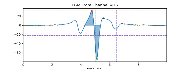
>>> ### egm of channel 16
>>> egmf, feat_names = sp.mea.egm_features(XE[16].copy(),act_loc=ATloc[16],fs=fs,plot=1,verbose=1,width_rel_height=0.75,
>>>                                     findex_rel_dur=1, findex_rel_height=0.3, findex_npeak=False,title='EGM From Channel #16')
    ------------------------------
    peak-to-peak (mV)  :     105.86761415086482
    duration  (samples):     28.314866535924523
    duration  (s)      :     0.001132594661436981
    duration  (ms)     :     1.132594661436981
    new duration (ms)  :     2.0126410178332197
    f-index     :    2
    ------------------------------