spkit.direction_flow_map
- spkit.direction_flow_map(X_theta, X=None, upsample=1, square=True, cbar=False, arr_pivot='mid', stream_plot=True, title='', heatmap_prop={}, arr_prop={'color': 'w', 'scale': None}, figsize=(12, 8), fig=None, ax=[], show=True, stream_prop={'color': 'k', 'density': 1}, **kwargs)
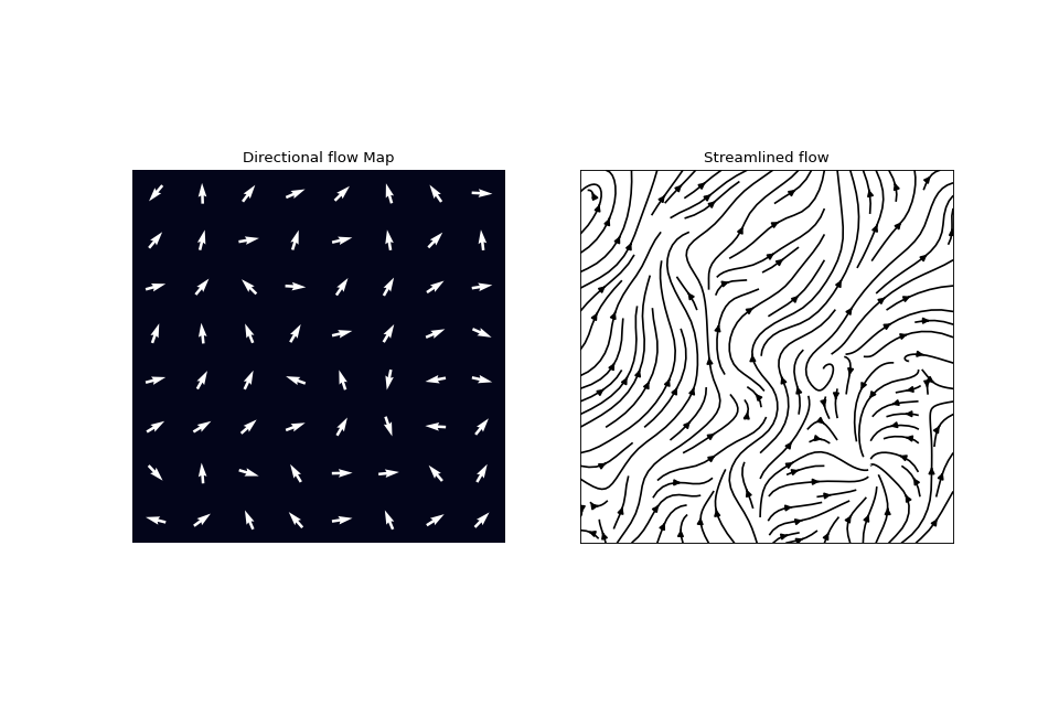
Displaying Directional flow map of a 2D grid
Displaying Directional flow map of a 2D grid
Displaying Directional Flow of a 2D grid, as spatial flow pattern.
- This plot two figures:
A 2D grid with arrows with a backgound of a heatmap
Streamline plot , if stream_plot=True
- Parameters:
- X_theta2D-array of Angles in Radian
2D Grid of Angles of direction at a point in a grid as spatial location, it can include NaN for missing information, or noisy location
- X2D-array of float, as size as X_theta, optional (default X=None)
These values are used as heatmap, behind the arrows of X_theta, if Not provided (X=None), X is created a grid of same size as X_theta with all values=0 to create a black background. X can be used as showing any related metrics of each directional arrow, such as confidance of computation, uncertainity of estimation, etc.
- square: bool, default=True,
Keep it True for correct aspect ratio of a Grid
- cbar: bool, Default=False
To show colorbar of heatmap, default is set to False
- arr_pivot: str, arrows location default=’mid’
This is used in plotting arrows, where location of arrow in a grid is plotted at the center Keeping it ‘mid’ is best to look on a uniform grid
- stream_plot: bool, Default=True
If set to True, a streamline plot of Directional flow is produced
- title: str, default=’’
To prepand a string on titles on both figures
- upsample: float, if greater than 1, X_theta is upsampled to new size of grid
that will entail:: new_size_of_grid = upsample*old_size_of_grid
- Properties to configure: Heatmap, Arrows and Streamline plot
- heatmap_prop: dict, properties for heatmap, default: heatmap_prop =dict()
properties of heatmap at background can be configured by using ‘heatmap_prop’ except for two keywords (square=True,cbar=False,) which are passed seprately, see above
- Some examples of settings
heatmap_prop =dict(vmin=0,vmax=20,cmap=’jet’,linewidth=0.01,alpha=0.1) heatmap_prop =dict(vmin=0,vmax=20,cmap=’jet’) heatmap_prop =dict(center=0)
- Some useful properties that can be changed are
(data, *, vmin=None, vmax=None, cmap=None, center=None, robust=False, annot=None, fmt=’.2g’, annot_kws=None, linewidths=0, linecolor=’white’, cbar_kws=None, cbar_ax=None, xticklabels=’auto’, yticklabels=’auto’)
for more details on heatmap_prop properties check https://seaborn.pydata.org/generated/seaborn.heatmap.html or help(seaborn.heatmap)
- arr_prop: dict, properties for arrow, default: arr_prop =dict(color=’w’,scale=None),
Properties of arrows can be configured using ‘arr_prop’, default color is set to white: ‘w’ except for ‘pivot’ keyword (pivot=’mid’), which is passed seprately, see above
- Some examples of settings
arr_prop =dict(color=’k’,scale=None) arr_prop =dict(color=’C0’,scale=30)
- Some useful properties that can be changed are
color: color of arrow width: Shaft width headwidthfloat, default: 3 headlengthfloat, default: 5 headaxislengthfloat, default: 4.5 minshaftfloat, default: 1 minlengthfloat, default: 1
for more details on heatmap_prop properties check https://matplotlib.org/stable/api/_as_gen/matplotlib.pyplot.quiver.html or help(plt.quiver)
- stream_prop:dict, properties for default: stream_prop=dict(density=1,color=’k’)
- Some examples of settings
stream_prop=dict(density=1,color=’k’) stream_prop=dict(density=2,color=’C0’)
- Some useful properties that can be changed are
(linewidth=None, color=None, cmap=None, norm=None, arrowsize=1, arrowstyle=’-|>’, minlength=0.1, transform=None, zorder=None, start_points=None, maxlength=4.0, integration_direction=’both’, broken_streamlines=True),
for more details on heatmap_prop properties check https://matplotlib.org/stable/api/_as_gen/matplotlib.pyplot.streamplot.html or help(plt.streamplot)
- figsize: tuple, default=(12,8): size of figure
- show: bool, default=True
If True, plt.show() is executed setting it false can be useful to change the figures propoerties
- ax: list of axis to use for plot, default =[]
Alternatively, list of axies can be passed to plot. if stream_plot=True, list of atleast two axes are expected, else atleast one if choosing stream_plot=False, still pass one axis as a list ax=[ax], rather than single axis itself If passed, ax[0] will be used for directional plot, and ax[1] will be used for streamplot, if stream_plot=True
- fig: deafult=None, if passing axes to plot, fig can be passed too, however, it is not used for anything other than returing
- Returns:
- X_theta: Same as input, if upsample>1, then new upsampled X_theta
- XSame as input, if upsample>1, then new upsampled X
If input was X=None, then returns X of 0
- (fig,ax): fig and ax, useful to change axis properties if show=False
See also
spkit#TODO
Notes
arr_prop = dict(scale=None,headwidth=None, headlength=None, headaxislength=None, minshaft=None, minlength=None,color=’w’)
Examples
>>> import numpy as np
>>> import matplotlib.pyplot as plt
>>> import spkit as sp
>>> np.random.seed(100)
>>> N,M = 8,8
>>> Ax_theta= np.arctan2(np.random.randn(N,M)+1, np.random.randn(N,M)+1)
>>> Ax_bad   = 1*(np.random.rand(N,M)>0.1).astype(float)
>>> Ax_bad[Ax_bad==0]=np.nan
>>> XY = sp.direction_flow_map(Ax_theta)
>>> plt.show()