spkit.mea.activation_repol_time_loc

spkit.mea.activation_repol_time_loc(X, fs=25000, at_range=[None, None], rt_range=[0.5, None], method='min_dvdt', gradient_method='fdiff', sg_window=11, sg_polyorder=3, gauss_window=0, gauss_itr=1, plot=False, plot_dur=2, **kwargs)

Computing Activation and Repolarisation Time together

Computing Activation Time and Repolarisation Time of multi-channel signals

Activation Time in cardiac electrograms refered to as time at which depolarisation of cells/tissues/heart occures. In contrast to ‘Activation Time’ in cardiac electrograms, Repolarisation Time, also refered as Recovery Time, indicates a time at which repolarisation of cells/tissues/heart occures.

For biological signals (e.g. cardiac electorgram), an activation time in signal is reflected by maximum negative deflection, which is equal to min-dvdt, if signal is a volatge signal and function of time x = v(t) and repolarisation time is again a reflected by maximum deflection (mostly negative), after activation occures.

However, simply computing derivative of signal is sometime misleads the activation and reoolarisation time location, due to noise, so derivative of a given signal has be computed after pre-processing. Repolarisation Time is often very hard to detect reliably, due to very small electrogram, which is mostly lost in noise.

Parameters:

Xnd-array

• Single Cycle of each channel containing EGM

• with shape = (nch,n),

• where nch: number of channels, n: number of samples,

fs: int, default=25000

• sampling frequency of signal,

t_range: list of [t0 (ms),t1 (ms)]

• range of time to restrict the search of activation time during t0 ms to t1 ms

• if t_range=[None,None], whole input signal is considered for search

• if t_range=[t0,None], excluding signal before t0 ms

• if t_range=[None,t1], excluding signal after t1 ms for search

rt_range: list of [t0 (ms),t1 (ms)]

• range of time to restrict the search of repolarisation time

• check spkit.get_activation_time and spkit.get_repolarisation_time for more details

method: str, default=”min_dvdt”

• Method to compute activation time

• one of (“max_dvdt”, “min_dvdt”, “max_abs_dvdt”)

• for more detail spkit.get_activation_time

gradient_method: str, default=’fdiff’

• Method to compute gradient of signal

• one of (“fdiff”, “fgrad”, “npdiff”,”sgdiff”,”sgdrift_diff”,”sgsmooth_diff”, “gauss_diff”)

• check spkit.signal_diff

Note

Same ‘method’ and ‘gradient_method’ is applied to both AT and RT computation.

To use different methods use spkit.get_activation_time and spkit.get_repolarisation_time seperatly

Parameters for gradient_method:

• used if gradient_method in one of (“sgdiff”,”sgdrift_diff”,”sgsmooth_diff”, “gauss_diff”)

• sg_window: sgolay-filter’s window length

• sg_polyorder: sgolay-filter’s polynomial order

• gauss_window: window size of gaussian kernel for smoothing,

• check help(signal_diff) from sp.signal_diff

plot:int, default=False

• If true, plot 3 figures for each channel

• 1. Full signal trace with activation time and repolarisation time

• 2. Segment of signal from loc-plot_dur to loc+plot_dur for activation time

• 3. Segment of signal from loc-plot_dur to loc+plot_dur for repolarisation time

• 4. Derivative of signal, with with activation time and repolarisation time

plot_dur: scalar, default=2,

• duration in seconds to plot, if plot=True

• segment of signal from loc-plot_dur to loc+plot_dur

• default=2s

gradient_method: Method to compute gradient of signal

one of (“fdiff”, “fgrad”, “npdiff”,”sgdiff”,”sgdrift_diff”,”sgsmooth_diff”, “gauss_diff”) check help(signal_diff) from sp.signal_diff

NOTE: Same ‘method’ and ‘gradient_method’ is applied to both AT and RT computation.

To use different methods use ‘get_activation_time’ and ‘get_repolarisation_time’ seperatly

Parameters for gradient_method:

used if gradient_method in one of (“sgdiff”,”sgdrift_diff”,”sgsmooth_diff”, “gauss_diff”)

sg_window: sgolay-filter’s window length sg_polyorder: sgolay-filter’s polynomial order gauss_window: window size of gaussian kernel for smoothing, check help(signal_diff) from sp.signal_diff

Returns:

at_loc: 1d-array

• array of length=nch, location of activation time as index

• to convert it in seconds, at_loc/fs

rt_loc: 1d-array

• array of length=nch, location of repolarisation time as index

• to convert it in seconds, rt_loc/fs

See also

spkit.get_activation_time, spkit.get_repolarisation_time, activation_time_loc

Examples

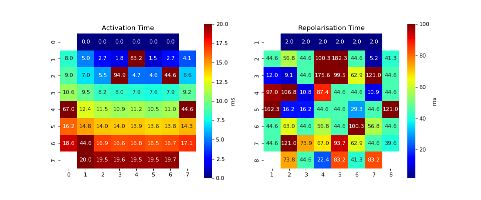
#sp.mea.activation_repol_time_loc
import numpy as np
import matplotlib.pyplot as plt
import os, requests
import spkit as sp

# Download Sample file if not done already

file_name= 'MEA_Sample_North_1000mV_1Hz.h5'

if not(os.path.exists(file_name)):
    path = 'https://spkit.github.io/data_samples/files/MEA_Sample_North_1000mV_1Hz.h5'
    req = requests.get(path)
    with open(file_name, 'wb') as f:
            f.write(req.content)

##############################
# Step 1: Read File
fs = 25000
X,fs,ch_labels = sp.io.read_hdf(file_name,fs=fs,verbose=1)

##############################
# Step 2: Stim Localisation
stim_fhz = 1
stim_loc,_  = sp.mea.get_stim_loc(X,fs=fs,fhz=stim_fhz, plot=0,verbose=0,N=None)

##############################
# Step 3: Align Cycles
exclude_first_dur=2
dur_after_spike=500
exclude_last_cycle=True

XB = sp.mea.align_cycles(X,stim_loc,fs=fs, exclude_first_dur=exclude_first_dur,dur_after_spike=dur_after_spike,
                        exclude_last_cycle=exclude_last_cycle,pad=np.nan,verbose=True)

print('Number of EGMs/Cycles per channel =',XB.shape[2])
##############################
# Step 4: Average Cycles

egm_number = -1

if egm_number<0:
    X1B = np.nanmean(XB,axis=2)
    print(' -- Averaged All EGM')
else:
    # egm_number should be between from 0 to 'Number of EGMs/Cycles per channel '
    assert egm_number in list(range(XB.shape[2]))
    X1B = XB[:,:,egm_number]
    print(' -- Selected EGM ->',egm_number)

print('EGM Shape : ',X1B.shape)

##############################
# Step 5-6: Activation and Repolarisation Time
at_range = [0,100]
rt_range = [2,100]

at_loc, rt_loc = sp.mea.activation_repol_time_loc(X1B,fs=fs,at_range=at_range, rt_range=rt_range)
at_loc_ms = 1000*at_loc/fs
rt_loc_ms = 1000*rt_loc/fs

print(at_loc_ms)
print(rt_loc_ms)
##############################
# Step 7: APD

apd_ms = rt_loc_ms-at_loc_ms

AT_grid = sp.mea.arrange_mea_grid(at_loc_ms, ch_labels=ch_labels)
RT_grid = sp.mea.arrange_mea_grid(rt_loc_ms, ch_labels=ch_labels)
APD_grid = sp.mea.arrange_mea_grid(apd_ms, ch_labels=ch_labels)
fig, ax = plt.subplots(1,2, figsize=(12,5))
sp.mea.mat_1_show(AT_grid,vmax=20, label = ('ms'),ax=ax[0])
ax[0].set_title('Activation Time')
sp.mea.mat_1_show(RT_grid,vmax=100,label = ('ms'),ax=ax[1])
ax[1].set_title('Repolarisation Time')
plt.show()

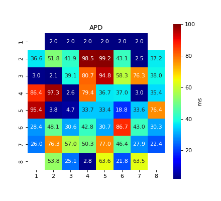
fig, ax = plt.subplots(figsize=(5.5,5))
sp.mea.mat_1_show(APD_grid,vmax=100, label = ('ms'),ax=ax)
ax.set_title('APD')
plt.show()

Examples using spkit.mea.activation_repol_time_loc

MEA: Step-wise Analysis: Example

MEA: Step-wise Analysis: Example