spkit.signal_diff
- spkit.signal_diff(x, method='fdiff', sg_window=101, sg_polyorder=1, gauss_window=0, gauss_itr=1, gauss_sigscale=2.7, dt=1)
Derivative of a signal
Derivative of a signal
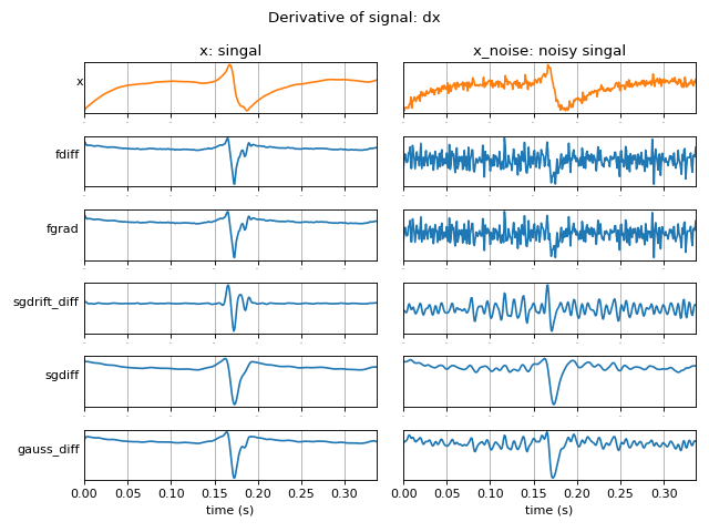
Computing Derivating of a signal is very useful in signal processing. In some of the physiological signals derivative of signal allows to compute events such as activation and repolarisation time.
This function implements some of the well known approaches to compute derivative
- ‘fdiff’:
Finite differentiation using first principle
intermediate values
\[dx(t) = [x(t+d) - x(t-d)]/2 \quad \text{when t+d and t-d in D (Domain)}\]boundries
first point t=0, when t+d in D, but t-d not in D
\[ \begin{align}\begin{aligned}dx(t) &= x(t+d)-x(t)\\dx(0) &= x(d)-x(0)\end{aligned}\end{align} \]last point t=l, when t-d in D, but t+d not in D
\[ \begin{align}\begin{aligned}dx(t) &= x(t)-x(t-d)\\dx(l) &= x(l)-x(l-d)\end{aligned}\end{align} \]- ‘fgrad’:
Finite differentiation
Using finite gradient (
np.gradient)
Note
fgradis essentially the same asfdiffcomputed in numpy usingnp.gradient- for following methods:
parameters for Savitzky-Golay filter (
sg_window,sg_polyorder)parameters for gaussian kernal+ConvFB (
gauss_window,gauss_itr), applied only ifgauss_window>0
- ‘sgdiff’:
Computing derivetive of signal using Savitzky-Golay filter,
then with gaussian kernal using Forward-Backward-Convolution (ConvFB).
- ‘sgdrift_diff’:
First remove drift using Savitzky-Golay filter,
then apply gaussian smoothing apply
fgrad.
- ‘sgsmooth_diff’:
First smooth the input signal x with Savitzky-Golay filter then apply
then apply gaussian smoothing (unnecessary, set
gauss_window =0to avoid) then applyfgrad
- ‘gauss_diff’:
First smooth the input signal x using gaussian smoothing
then apply
fgrad
- ‘npdiff’:
npdiff uses numpy’s
np.diff, which computes x[n+1] - x[n]for compleness, npdiff is included.
- Parameters:
- x: 1d-array signal
- method: method to compute derivative, one of the above
- (sg_window,sg_polyorder,gauss_window,gauss_itr): Savitzky-Golay filter, Gaussian smoothing using Forward-Backward-Convolution (ConvFB)
- Returns:
- dx: derivative of signal
Notes
Using fdiff and fgrad results in same output.
for noisy signal, applying smoothing first is always recommonded, (see example below)
References
For Noisy signal, one of the other approach is using Total Variation - https://arxiv.org/pdf/1701.00439
Examples
#sp.signal_diff
import numpy as np
import matplotlib.pyplot as plt
import spkit as sp
x, fs = sp.data.optical_sample(sample=2)
x = x[int(0.023*fs):int(0.36*fs)]
x = x - x.mean()
x_noise = sp.add_noise(x,snr_db=10)
t = np.arange(len(x))/fs

methods = ['fdiff','fgrad','sgdrift_diff','sgdiff','gauss_diff']
DX1 = [sp.signal_diff(x.copy(),method=method,sg_window=11,gauss_window=11) for method in methods]
DX2 = [sp.signal_diff(x_noise.copy(),method=method,sg_window=11,gauss_window=11) for method in methods]

figsize = (8,6)
K = len(DX1)

plt.figure(figsize=figsize)
plt.subplot(K+1,2,1)
plt.plot(t,x,'C1')
plt.xlim([t[0],t[-1]])
plt.ylabel(f'x',rotation=0)
plt.yticks([])
plt.xticks(fontsize=0)
plt.grid()
plt.title(f'x: singal')

plt.subplot(K+1,2,2)
plt.plot(t,x_noise,'C1')
plt.xlim([t[0],t[-1]])
#plt.ylabel(f'x')
plt.yticks([])
plt.xticks(fontsize=0)
plt.grid()
plt.title(f'x_noise: noisy singal')

for i in range(K):
    plt.subplot(K+1,2,i*2+3)
    plt.plot(t[:len(DX1[i])],DX1[i],color='C0')
    plt.xlim([t[0],t[-1]])
    plt.grid()
    plt.yticks([])
    #plt.xticks(labels='')
    plt.ylabel(methods[i],rotation=0, ha='right')
    if i==K-1:
        plt.xlabel('time (s)')
    else:
        plt.xticks(fontsize=0)

    plt.subplot(K+1,2,i*2+4)
    plt.plot(t[:len(DX2[i])],DX2[i],color='C0')
    plt.xlim([t[0],t[-1]])
    plt.grid()
    #if i<K-1:plt.xticks([])
    plt.yticks([])
    #plt.ylabel(f'$N={N[i]}$')
    #plt.legend(frameon=False,bbox_to_anchor=(1,1))
    if i==K-1:
        plt.xlabel('time (s)')
    else:
        plt.xticks(fontsize=0)

plt.suptitle('Derivative of signal: dx')
plt.subplots_adjust(hspace=0,wspace=0.05)
plt.tight_layout()
plt.show()


