spkit.mea.analyse_mea_file

spkit.mea.analyse_mea_file(file_name, stim_fhz, fs=25000, egm_number=-1, dur_after_spike=None, exclude_first_dur=2, exclude_last_cycle=True, repol_computation=False, bad_ch_stim_thr=2, bad_ch_mnmx=[None, None], p2p_thr=5, range_act_thr=[0, 50], bad_channels=[], good_channels=[], max_volt=1000, verbose=1, **kwargs)

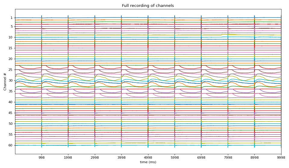
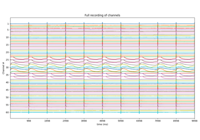
A Complete Analysis of a MEA recording

A Complete Analysis of a MEA recording

Given a MEA recoring file in HDF formate (‘.h5’), a complete analysis is provided, step-wise. This function can be used to analyse 100s of files with same paramter settings. Function returns all the feature computed as a DataFrame, with can be exported as csv file

There are many different parameters to set at each step, some of them can be configured via input argumets. The deafult setting of all the parameters at each steps are choosen as to work well for observed cases. For full analysis, try each step seprately to optimise parameters for your own file, once, they are determined, 100s of files can be analysed and same save all the computed metrics in a csv/excel file.

                MEA 8x8 GRID

    | 21 | 31 | 41 | 51 | 61  | 71 |

|12 | 22 | 32 | 42 | 52 | 62  | 72 | 82 |

|13 | 23 | 33 | 43 | 53 | 63  | 73 | 83 |

|14 | 24 | 34 | 44 | 54 | 64  | 74 | 84 |

|15 | 25 | 35 | 45 | 55 | 65  | 75 | 85 |

|16 | 26 | 36 | 46 | 56 | 66  | 76 | 86 |

|17 | 27 | 37 | 47 | 57 | 67  | 77 | 87 |

    | 28 | 38 | 48 | 58 | 68  | 78 |

Parameters:

file_name: str,

• file name with full accessible path. File should be in .h5 format. If you have bdf file, use Multichannel Data Manager to cover file type.

  check here, how to convert bdf to hdf file: Multichannel Data Manager: https://www.multichannelsystems.com/software/multi-channel-datamanager

stim_fhz(float, int)

• Frequency of Stimulus in Hz (cycles per seconds): eg. 1, 2 etc

• for 1Hz, stim_fhz =1

• Setting stim_fhz=None

  if stim_fhz=None, it tries to extract it from file name, if exist, else error will be raised for example, if file_name=’MEA_North_1000_1Hz.h5’ function will extract ‘1Hz’ and set stim_fhz=1 This is useful, if analysing mutiple files, with different Frequency of stimulus

fsint, default=25000 (= 25KHz)

• Sampling Frequency of MEA recording

max_volt: float, int, default=1000

• Maximum voltage of signal or stimuli recorded Default datatype of signal recoridng in HDF file is usually ‘int32’, which leades to range from -32768 to 32767 if max_volt=None, then unnormalised signal values are returned. if max_volt is not None, then return signal values will be float32 and from -max_volt to max_volt

  Note

  If max_volt is changed, make sure to adjust all the other parameters.

verbose: int, default=1

• level of verbosity,

• heigher it is more details computations are printed on consol

• 0 Silent

• 1 a few details

• 2 a little more computations

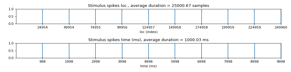
Stim loc

stim_id_param: dict,

• default

stim_id_param = dict(method='max_dvdt',gradient_method='fdiff',
        ch=0,N=None,plot=0,figsize=(12,3))

• Parameter setting to identify stimuli locations

  • method: str, default=’max_dvdt’

    • stim location as maximum deflection, which occures when stim shift from -ve to +ve voltage

  • gradient_method ='fdiff': finite differentiation

  • ch=0: fist chennel to id stim loc

  • plot=0: if to plot, with figsize=(12,3)

• check get_stim_loc for details

Aligning Cycles

exclude_first_durfloat, default=2 (ms)

• Exclude the duration (in ms) of signal after stimulus spike loc, default 1 ms

• It depends on the method of finding stim loc, since stim is 1ms -ve, 1ms +v, and loc is

• detected as middle transaction (max_dvdt), atleast 1ms of duration should be excluded.

• Default 2ms is excluded, to be safe side

dur_after_spikefloat, int, default=None

• Extract the duration (in ms) after stimulus spike loc to search for EGM

• If set to None (default), dur_after_spike is computed based on stimuli frequency (stim_fhz)

  • stim_fhz = 1 –> dur_after_spike = 500

  • stim_fhz = 2 –> dur_after_spike = 300

  • stim_fhz = 3 –> dur_after_spike = 250

  • stim_fhz > 3 –> dur_after_spike = 200

exclude_last_cycle: bool, default=True,

• If True, last cycle of stimuli is excluded while aligning cycles. It is recommonded to exclude last egm, as sometimes, last egm might shorter than other, which produces artifact while averaging.

Averaging or Selecting EGM/Cycle

egm_numberint, (>=-1), default=-1

• EGM number (cycle number of stimuli) to be analysed. Number start from 0, to number of cycles of stimuli

• egm_number = 0 for analysing 1st EGM of 1st cycle, 1, 2 for 2nd and 3rd and so on,

• if egm_number=-1 is passed, all the EGMs are averaged first, before analysing, which is often a good idea to cancel out noise

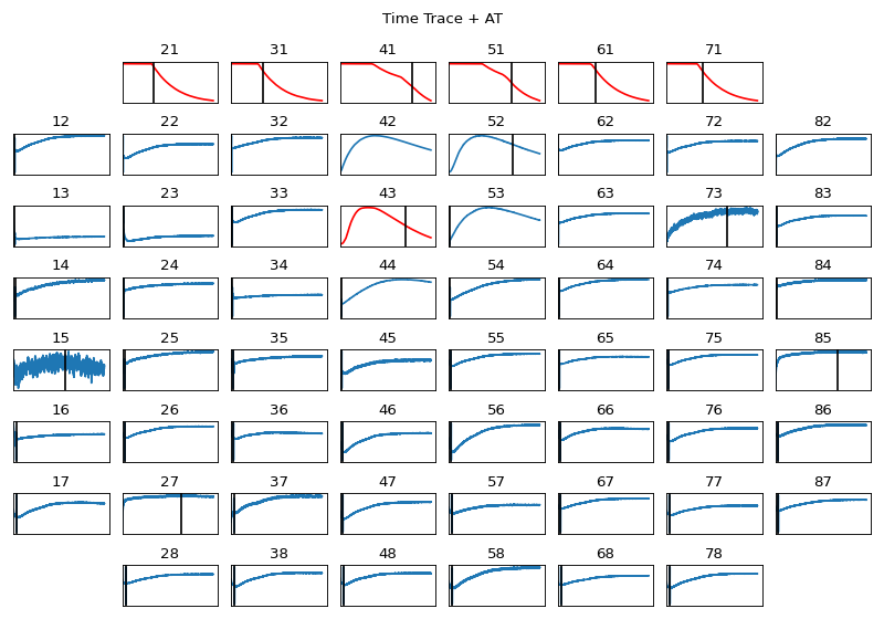
Activation & Repolarisation Time Localisation

repol_computation: bool, default=False,

• if True, repolarisation time is computed, which leads to computation of APD = RT-AT

• if True, parameter setting from ‘at_id_param’ is used

at_id_param: dict

• Parameters to compute activation and repolarisation time loc

• Default

at_id_param= dict(at_range=[0,None],rt_range= [0.5, None],
              method='min_dvdt',gradient_method='fdiff',
              sg_window= 11,sg_polyorder=3,
              gauss_window=0,gauss_itr=1,
              plot=False,plot_dur=2)

at_range: list of two [t0,t1] default=[0,None], in ms

time limitation in which AT is to be searched, t0 ms to t1 ms limiting it can improve the results

for more detail check: spkit.get_activation_time

rt_range: list of two [t0,t1] default=[0.5, None], in ms

Only used if repol_computation =True time limitation for repolarisation, AFTER activation time Recommended to use t0 = 0.5, after 0.5 ms of activation time, search for RT

for more detail check: spkit.get_repolarisation_time

parameters to identify location

• method='min_dvdt' : For activation and repolarisation minimum deflection, which is maximum -ve deflection is used,

• gradient_method='fdiff': finite differentiation of signal

• (sg_window= 11,sg_polyorder=3,gauss_window=0,gauss_itr=1), used if gradient_method other than ‘fdiff’

• plot=False, if True, plot AT & RT

• plot_dur=2, used plot is True

for more detail check: activation_time_loc, activation_repol_time_loc

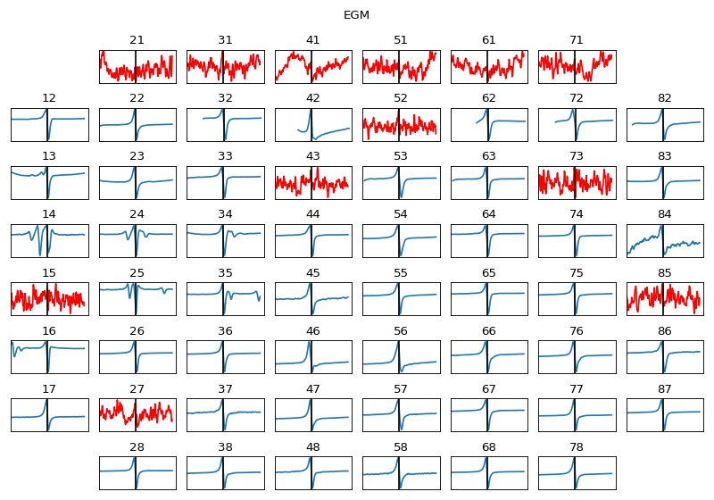
Exctracting EGM

egm_id_param: dict,

• Parameters used while exctracting EGM from each channel.

• Default setting

  egm_id_param = dict(dur_from_loc=5,remove_drift=True,
                     apply_after=True,sg_window=201,
                     sg_polyorder=1,pad=np.nan,
                     verbose=0,plot=False)
  

for more detail check: func:extract_egm

Given activation location for EGM, two type of parameters are required (1) duration of EGM to be extracted, and (2) preprocessing EGM

• dur_from_loc: float, default=5 ms

  From given loc, dur_from_loc ms from both side of signal is extract, as EGM if dur_from_loc=5, then 10ms of eletrogram is extracted

• remove_drift: bool, default=True,

  If True, Savitzky-Golay filter is applied to remove the drift

• apply_after: bool, default=True,

  If True, Savitzky-Golay filter to remove drift is applied after extracting EGM Else drift is removed from entire signal and EGM is extracted

• Parameters for Savitzky-Golay filter

  : sg_window=91,sg_polyorder=1 : keep the window size large enough and polyorder low enough to remove only drift

Note

Parameters of Savitzky-Golay filter should be choosen appropriately, which depends if

it is applied before or after extracting EGM. In case of after EGM extraction, signal is a small length, so need to adjust sg_window accordingly

• pad: default=np.nan

  To pad values to EGM, in case is to shorter than others. Padding is done to make all EGMs of same shape-nd-array

• plot: bool, default False

  If True, two figures per channel are plotted Figure 1 shows, a raw EGM, computed drift and corrected EGM Figure 2 shows, Only corrected EGM with loc

• verbose: bool, default=False

  If True, intermediate computations are printed,

Feature Exctracting from EGM

egm_feat_param: dict,

• Parameters to extract Features from EGM

• Default setting .. code-block:

  egm_feat_param = dict(width_rel_height=0.75,
             findex_rel_dur=0.5,
             findex_rel_height=0.75,
             findex_npeak=False,
             plot=0,verbose=0)
  

  for more detail check: func:egm_features

• There are 7 features extracted from each EGM

  1. Peak to Peak voltage

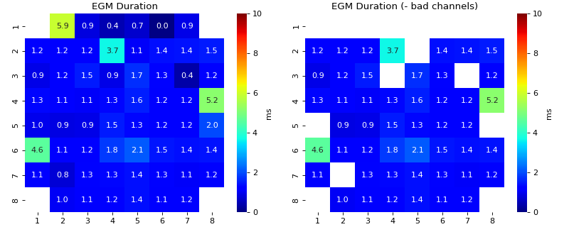
  2. Duration of EGM

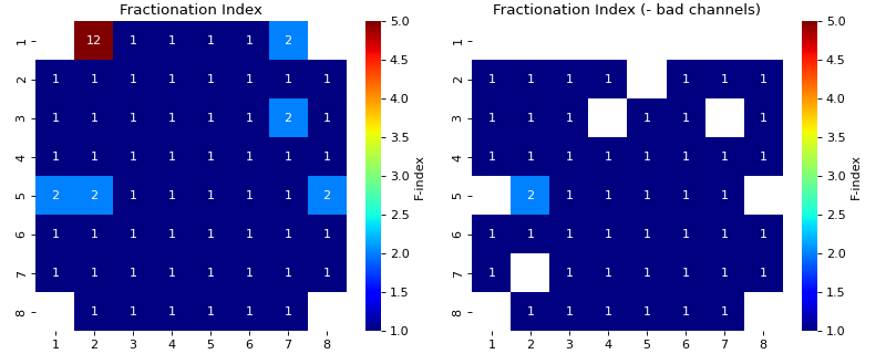
  3. Fractional Index

  4. Refined Duration of EGM based on fractionating peaks

  5. Energy of EGM

  6. Voltage Dispersion

  7. Noise variance

  For detailed overview of all the feature check: egm_features

• width_rel_height: scalar, default=0.75

  • Relative hight of peaks to estimate the width of peaks,

  • Lower it is smaller the width of peak be, which leads to smaller duration of EGM

• findex_rel_dur: +ve scalar, default = 1

  • Relative duration of search region, to find fractionating peaks.

  • As explained above for duration,

• findex_rel_height: scalar, default=0.75

  • Relative height threshold for defining the fractionation,

  • Any positive peak which exceeds the hight of 0.75*positive peak of EGM at loc, within Search region is considered fractionating peak

  • Similarly, any negative peak which goes below 0.75*negative peak of EGM at loc, within Search region is considered fractionating peak

• findex_npeak: bool, deafult=False

  • if true, negative peaks are considered for fractionation, default=False

• plot: if True,

  plot EGM with all the features shown

• figsize=(8,3): size of figure

• verbose: 0 Silent

  1 a few details 2 all the computations

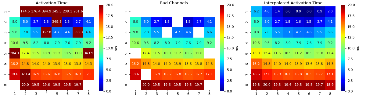
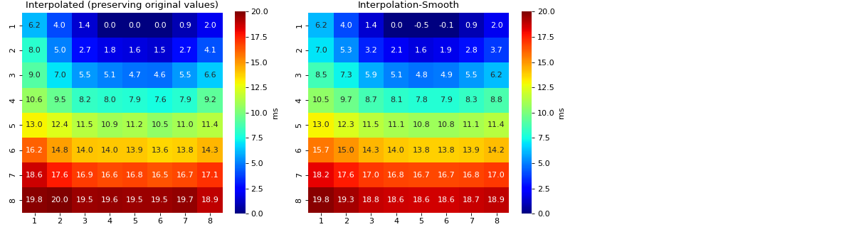
Interpolation of Feature Matrix - AT

intp_param: dict,

• default setting

  intp_param = dict(pkind='linear',filter_size=3,method='conv')
  

• Parameters used for interpolating Activation Map

  • pkind='linear': kind of interpolation

  • filter_size=3: filter_size to smooth the map,

  • method='conv': method of convolution

  Note

  Increase ‘filter_size’ for more smoother MAP

for more details check spkit.fill_nans_2d

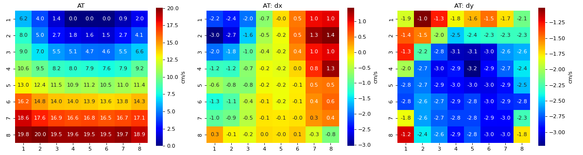
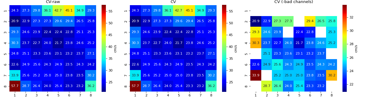
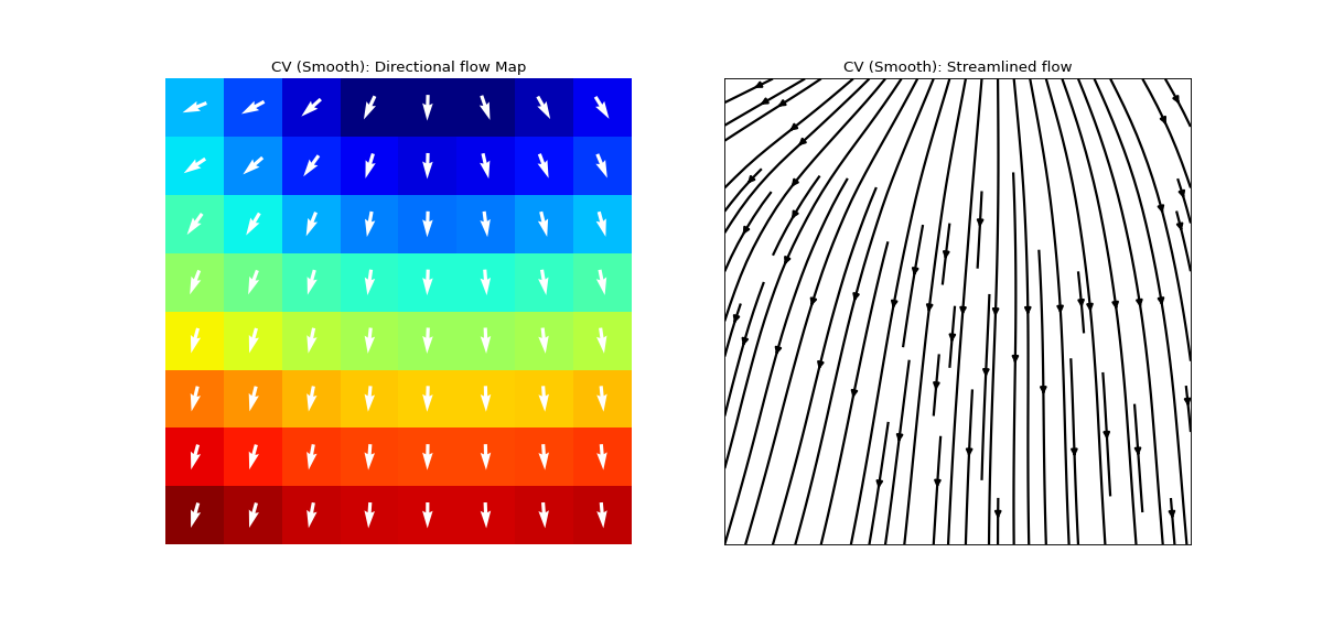
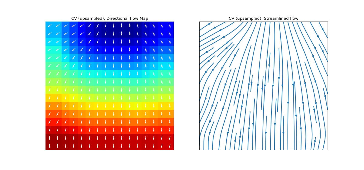
Conduction Velocity computation

cv_param: dict,

• Parameter setting to compute Conduction Velocity

• Default setting

  cv_param = dict(eD=700,esp=1e-10,cv_pad=np.nan,
                cv_thr=100,arr_agg='mean',
                plots=2,verbose=True)
  

eD: scaler, (default=700 mm)

• Inter-Node Distance

• distance between two nodes in horizontal and vertical axis on MEA electrode-plate distance is given in mm

esp: scalar, default =1e-10

• epsilon

• to avoid diving by zero, esp is used

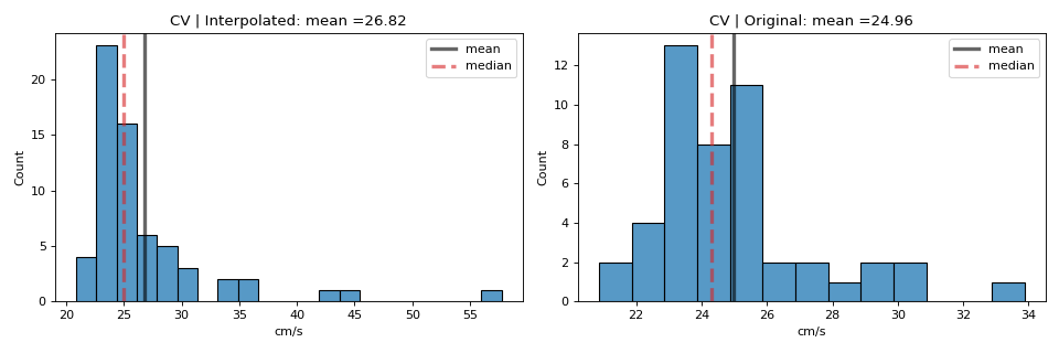
cv_thr: scalar, default=100 cm/s

• threshold on conduction velocity to exclude

• any electrodes shows cv>=cv_thr is replaced by ‘cv_pad’ (np.nan)

cv_pad: scalar default=np.nan

• replacement value

• any cv value above cv_thr is replaced by cv_pad, to avoid including in computation

arr_agg: str, {‘mean’,’median’} default=’mean’

• method to aggregate the directional arrows, mean or median

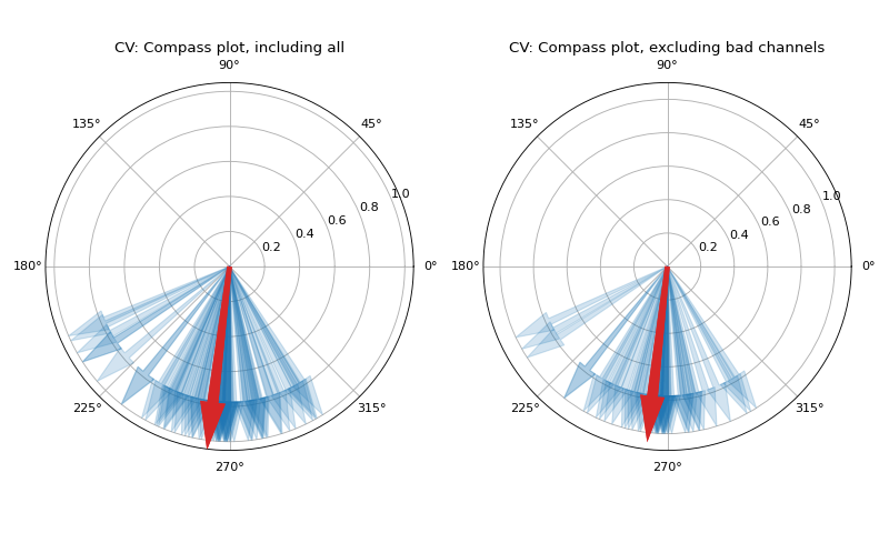
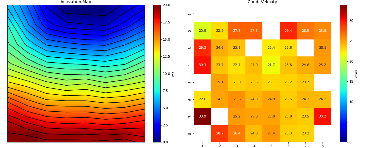
plots: int, default=1

• if 1, plot two figures for CV maps, two figures for directional compass

• if 2, also plot activation matrix and conduction velocity matrix with more details

verbose: boot, default=True

• verbosity

• print information

For more details check compute_cv

Identifying Bad Channels & Bad EGMs

1. Based on Stimulus duration

• If stimulus last longer than threshold duration, given by ‘bad_ch_stim_thr’ in ms

• bad_ch_thr: float, default = 2 (ms)

  • Duration, if average duration of stimuli per cycle exceed the threshold on either side +ve/-ve, it is flagged as bad channel

  Note

  Lower the threshold, more channels will be flagged, higher the threshold less channels will be flagged

• bad_ch_mnmx: list of two [None, None]

  • minimum and maximum valtage of stimulus, e.g. -1000, 1000.

  • Default is None, in which case, it is computed from min and max of signal itself.

  • Increase this threhold to avoid flagging channels as bad.

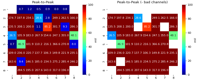
for more details, check find_bad_channels_idx

2. Based on EGM voltage

• If EGM is very small, it is usually a noise

• p2p_thrfloat, default=5,

  • Threhold on peak-to-peak voltage of EGM, if EGM has less the threshold peak-to-peak, it is flagged as bad

  • Descrese this threhold to avoid flagging channels as bad.

  Note

  Lower the threshold, less channels will be flagged, higher the threshold more channels will be flagged

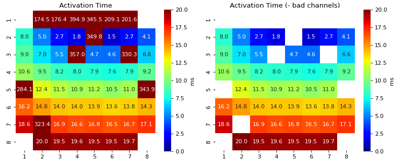
3. Based on Activation Time

• If activation time is out of given range

• range_act_thr: list of two, deafult = [0, 50],

  • Minimum and maximum activation time range. If activation time of EGM is out of given limits, then it is flagged as bad.

  • By dfault, if activation time is greater than zero, it is considered okay.

  • Example, range_act_thr = [5,30] means, if activation time is less than 5 ms or grater than 30 ms, is it flagged as bad

  • range_act_thr = [0,30] works well too

• Manually passing list of channels as BAD and GOOD

  Passing list of good and bad channels overrides the criteria mentioned above, and enforces the list of Good and Bad

  • bad_channels: list, deafault = []

    • Passing list of bad channels ensures that channel is in list of bad channels, regardless of criteria

    • For example, channel 15 is alwasy a bad so bad_channels=[15]

    • List should have same name of channels as in channel labels

  • good_channels: list, deafault = []

    • Passing list of good channels overrides the criteria mentioned above, and exclude them from list of bad channels

    • List should have same name of channels as in channel labels

Settings for All the plots

• map_prop: dict,

  • Customising ranges for heatmap, colormap, style, type of objects to plot

  Default setting

  map_prop = dict(at_range=[0,20],p2p_range=[0,100],
             dur_range=[0,10],f_range=[1,5],
             cv_range=[0,None],rt_range=[0,100],
             apd_range=[0,50],at_cmap='jet',
             interpolation='bilinear',countour_n=25,
             countour_clr='k',
             cv_arr_prop = dict(color='w',scale=None))
  

  Ranges of plot colormaps Final Activation Map with countours

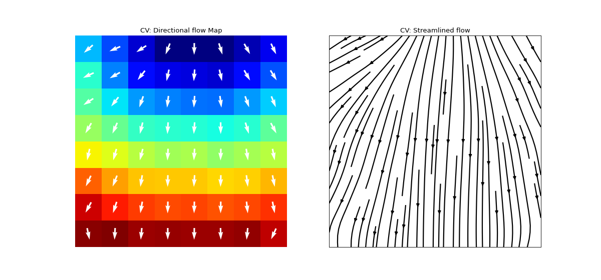
  Conducntion Velocity Arrows

  • cv_arr_prop=dict(color=’w’,scale=None)

  for more details check spkit.direction_flow_map

Returns:

Features_dfpd.dataframe,

• Statistics of all the features (mean, median, sd across all the channels)

Features_chFeatures of all the channels

Features_matFeature Matrices of Activation Time, Conduction Velocity, Bad Channel etc

Data: dict of signal, channel labes and fs

• i.e. {‘X’:X, ‘ch_labels’:ch_labels, ‘fs’:fs}

See also

get_stim_loc, align_cycles, activation_time_loc, activation_repol_time_loc, extract_egm, egm_features

Notes

Check [Examples](https://spkit.github.io/auto_examples/) tab

A code that shows full parameter settings

#parameters
stim_id_param = dict(method='max_dvdt',gradient_method='fdiff',
                 ch=0,N=None,plot=0,figsize=(12,3))

at_id_param  = dict(at_range=[0,None],rt_range= [0.5, None],method='min_dvdt',
                gradient_method='fdiff',sg_window= 11,sg_polyorder=3,
                gauss_window=0,gauss_itr=1,plot=False,plot_dur=2)

egm_id_param = dict(dur_from_loc=5,remove_drift=True,apply_after=True,
                    sg_window=201,sg_polyorder=1,pad=np.nan,
                    verbose=0,plot=False)

egm_feat_param = dict(width_rel_height=0.75,findex_rel_dur=0.5,
                    findex_rel_height=0.75,findex_npeak=False,
                    plot=0,verbose=0)

intp_param = dict(pkind='linear',filter_size=3,method='conv')
cv_param = dict(eD=700,esp=1e-10,cv_pad=np.nan,cv_thr=100,arr_agg='mean',plots=2,
               verbose=True)
map_prop = dict(at_range=[0,20],p2p_range=[0,100],dur_range=[0,10],f_range=[1,5],
                cv_range=[0,None],rt_range=[0,100],apd_range=[0,50],
                at_cmap='jet',interpolation='bilinear',countour_n=25,
                countour_clr='k',cv_arr_prop = dict(color='w',scale=None))

#final-call
Fdf,Fch,Fmat,Data = sp.mea.analyse_mea_file(file_name, stim_fhz, fs=25000, egm_number=-1, 
                dur_after_spike=None, exclude_first_dur=2, exclude_last_cycle=True, 
                repol_computation=False, bad_ch_stim_thr=2, bad_ch_mnmx=[None, None], 
                p2p_thr=5, range_act_thr=[0, 50], bad_channels=[], good_channels=[], max_volt=1000,
                verbose=1, stim_id_param=stim_id_param,at_id_param=at_id_param,
                egm_id_param=egm_id_param, egm_feat_param=egm_feat_param,intp_param=intp_param,
                cv_param=cv_param,map_prop=map_prop)

Examples

>>> #sp.mea.analyse_mea_file
>>> import numpy as np
>>> import matplotlib.pyplot as plt
>>> import os, requests
>>> import spkit as sp
>>> print('spkit-version: ',sp.__version__)
>>> # Download Sample file if not done already
>>> file_name= 'MEA_Sample_North_1000mV_1Hz.h5'
>>> if not(os.path.exists(file_name)):
>>>     path = 'https://spkit.github.io/data_samples/files/MEA_Sample_North_1000mV_1Hz.h5'
>>>     req = requests.get(path)
>>>     with open(file_name, 'wb') as f:
>>>             f.write(req.content)
>>> Features_df,Features_ch,Features_mat, Data = sp.mea.analyse_mea_file(file_name,stim_fhz=1)

Examples using spkit.mea.analyse_mea_file

MEA: Minimal Setting: Example

MEA: Minimal Setting: Example