Note
Go to the end to download the full example code or to run this example in your browser via JupyterLite or Binder
Release Highlights for spkit 0.0.9.7
Release Highlights for spkit 0.0.9.7
We are pleased to announce the release of spkit 0.0.9.7, which comes with many fixed bug, more organised documentation and new features! For an exhaustive list of all the changes, please refer to the release notes.
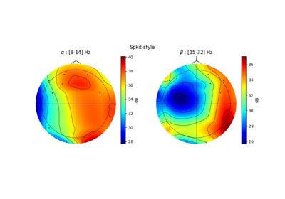
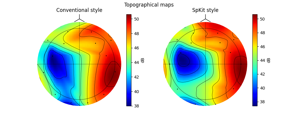
Topographic Map correction: 10-20 System
A widely used EEG system is 10-20 system, although there are many libraries that can plot topographic map from EEG data, their layouts are a little different than standards.
Notice the 10-20 Standard described in following
In above examples, Cz is the center point and horizontal line crossing is straight line. In Spkit we tried to correct this mapping style, however, keeping the conventional style as option. See following examples.
#sp.eeg.topomap
import numpy as np
import matplotlib.pyplot as plt
import spkit as sp
X,fs, ch_names = sp.data.eeg_sample_14ch()
X = sp.filterDC_sGolay(X, window_length=fs//3+1)
Px,Pm,Pd = sp.eeg.rhythmic_powers(X=X,fs=fs,fBands=[[4],[8,14]],Sum=True,Mean=True,SD =True)
Px = 20*np.log10(Px)
pos1, ch = sp.eeg.s1020_get_epos2d(ch_names,style='eeglab-mne')
pos2, ch = sp.eeg.s1020_get_epos2d(ch_names,style='spkit')
fig, ax = plt.subplots(1,2,figsize=(10,4))
Z1i,im1 = sp.eeg.topomap(pos=pos1,data=Px[1],axes=ax[0],return_im=True)
Z2i,im2 = sp.eeg.topomap(pos=pos2,data=Px[1],axes=ax[1],return_im=True)
ax[0].set_title(r'Conventional style')
ax[1].set_title(r'SpKit style')
plt.colorbar(im1, ax=ax[0],label='dB')
plt.colorbar(im2, ax=ax[1],label='dB')
plt.suptitle('Topographical maps')
plt.show()
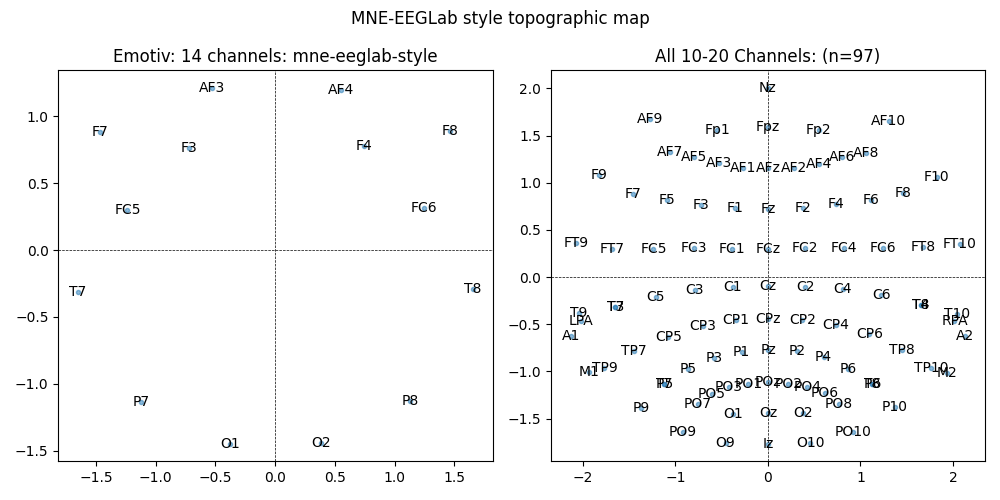
Location of all the eletrodes
Location of all the electrodes are shown here.
import numpy as np
import matplotlib.pyplot as plt
import spkit as sp
ch_names_emotiv = ['AF3','F7','F3','FC5','T7','P7','O1','O2','P8','T8','FC6','F4','F8','AF4']
pos1, ch1 = sp.eeg.s1020_get_epos2d(ch_names_emotiv)
pos2, ch2 = sp.eeg.s1020_get_epos2d(ch_names_emotiv,style='spkit')
ch_names_all = sp.eeg.presets.standard_1020_ch
pos3, ch3 = sp.eeg.s1020_get_epos2d(ch_names_all)
ch_names_spkit_all = sp.eeg.presets.standard_1020_spkit_ch
pos4, ch4 = sp.eeg.s1020_get_epos2d(ch_names_spkit_all,style='spkit')
plt.figure(figsize=(10,5))
plt.subplot(121)
plt.plot(pos1[:,0],pos1[:,1],'.',alpha=0.5)
for i,ch in enumerate(ch_names_emotiv):
plt.text(pos1[i,0],pos1[i,1],ch,va='center',ha='center')
plt.title('Emotiv: 14 channels: mne-eeglab-style')
plt.axvline(0,lw=0.5,color='k',ls='--')
plt.axhline(0,lw=0.5,color='k',ls='--')
plt.subplot(122)
plt.plot(pos3[:,0],pos3[:,1],'.',alpha=0.5)
for i,ch in enumerate(ch_names_all):
plt.text(pos3[i,0],pos3[i,1],ch,va='center',ha='center')
plt.title(f'All 10-20 Channels: (n={len(ch_names_all)})')
plt.axvline(0,lw=0.5,color='k',ls='--')
plt.axhline(0,lw=0.5,color='k',ls='--')
plt.suptitle('MNE-EEGLab style topographic map')
plt.tight_layout()
plt.show()
plt.figure(figsize=(10,5))
plt.subplot(121)
plt.plot(pos2[:,0],pos2[:,1],'.',alpha=0.5)
for i,ch in enumerate(ch_names_emotiv):
plt.text(pos2[i,0],pos2[i,1],ch,va='center',ha='center')
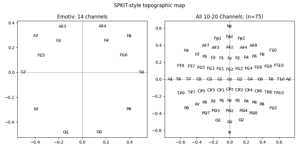
plt.title('Emotiv: 14 channels')
plt.axvline(0,lw=0.5,color='k',ls='--')
plt.axhline(0,lw=0.5,color='k',ls='--')
plt.subplot(122)
plt.plot(pos4[:,0],pos4[:,1],'.',alpha=0.5)
for i,ch in enumerate(ch_names_spkit_all):
plt.text(pos4[i,0],pos4[i,1],ch,va='center',ha='center')
plt.title(f'All 10-20 Channels: (n={len(ch_names_spkit_all)})')
plt.suptitle('SPKIT-style topographic map')
plt.axvline(0,lw=0.5,color='k',ls='--')
plt.axhline(0,lw=0.5,color='k',ls='--')
plt.tight_layout()
plt.show()
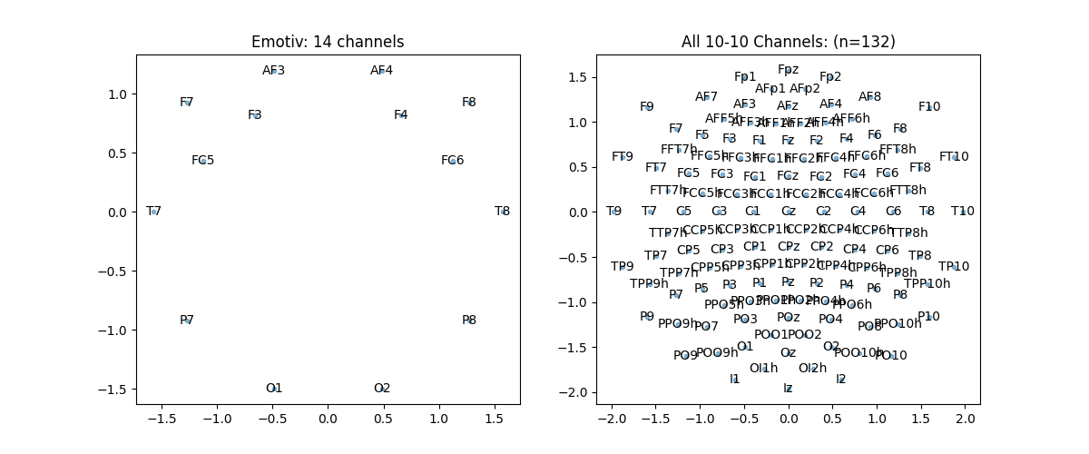
Topographic Map 10-10 System
import numpy as np
import matplotlib.pyplot as plt
import spkit as sp

ch_names = ['AF3','F7','F3','FC5','T7','P7','O1','O2','P8','T8','FC6','F4','F8','AF4']
pos, ch = sp.eeg.s1010_get_epos2d(ch_names)

plt.figure(figsize=(12,5))

plt.subplot(121)
plt.plot(pos[:,0],pos[:,1],'.',alpha=0.5)
for i,ch in enumerate(ch_names):
    plt.text(pos[i,0],pos[i,1],ch,va='center',ha='center')
plt.title('Emotiv: 14 channels')

ch_names = sp.eeg.presets.standard_1010_ch
pos, ch = sp.eeg.s1010_get_epos2d(ch_names)

plt.subplot(122)
plt.plot(pos[:,0],pos[:,1],'.',alpha=0.5)
for i,ch in enumerate(ch_names):
    plt.text(pos[i,0],pos[i,1],ch,va='center',ha='center')
plt.title(f'All 10-10 Channels: (n={len(ch_names)})')
plt.show()
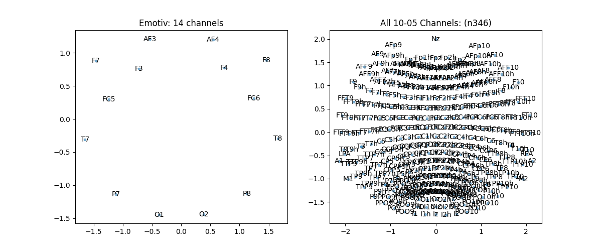
Topographic Map 10-05 System
import numpy as np
import matplotlib.pyplot as plt
import spkit as sp

ch_names = ['AF3','F7','F3','FC5','T7','P7','O1','O2','P8','T8','FC6','F4','F8','AF4']
pos, ch = sp.eeg.s1005_get_epos2d(ch_names)

plt.figure(figsize=(12,5))

plt.subplot(121)
plt.plot(pos[:,0],pos[:,1],'.',alpha=0.5)
for i,ch in enumerate(ch_names):
    plt.text(pos[i,0],pos[i,1],ch,va='center',ha='center')
plt.title('Emotiv: 14 channels')

ch_names = sp.eeg.presets.standard_1005_ch
pos, ch = sp.eeg.s1005_get_epos2d(ch_names)

plt.subplot(122)
plt.plot(pos[:,0],pos[:,1],'.',alpha=0.5)
for i,ch in enumerate(ch_names):
    plt.text(pos[i,0],pos[i,1],ch,va='center',ha='center')
plt.title(f'All 10-05 Channels: (n{len(ch_names)})')
plt.show()
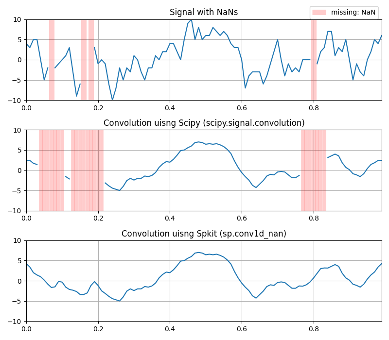
Convolution with missing values (NaNs)
- 1D
sp.conv1d_nan
import numpy as np
import matplotlib.pyplot as plt
import scipy
import spkit as sp
seed = 4
x = (sp.create_signal_1d(n=100,seed=seed,sg_winlen=5)*10).round(0)
t = np.arange(len(x))/100
np.random.seed(seed)
r = np.random.rand(*x.shape)
x[r<0.05] = np.nan
kernel = np.ones(7)/7
np.random.seed(None)
x_scipy = scipy.signal.convolve(x.copy(), kernel,mode='same')
x_spkit = sp.conv1d_nan(x.copy(), kernel)
plt.figure(figsize=(8,7))
plt.subplot(311)
plt.plot(t,x,color='C0')
plt.vlines(t[np.isnan(x)],ymin=np.nanmin(x),ymax=np.nanmax(x),color='r',alpha=0.2,lw=8,label='missing: NaN')
plt.xlim([t[0],t[-1]])
plt.ylim([np.nanmin(x),np.nanmax(x)])
plt.legend(bbox_to_anchor=(1,1.2))
plt.grid()
plt.title('Signal with NaNs')
plt.subplot(312)
plt.plot(t,x_scipy)
plt.vlines(t[np.isnan(x_scipy)],ymin=np.nanmin(x),ymax=np.nanmax(x),color='r',alpha=0.2,lw=5.5)
plt.xlim([t[0],t[-1]])
plt.ylim([np.nanmin(x),np.nanmax(x)])
plt.grid()
plt.title('Convolution uisng Scipy (scipy.signal.convolution)')
plt.subplot(313)
plt.plot(t,x_spkit)
plt.xlim([t[0],t[-1]])
plt.ylim([np.nanmin(x),np.nanmax(x)])
plt.grid()
plt.title('Convolution uisng Spkit (sp.conv1d_nan)')
plt.tight_layout()
plt.show()
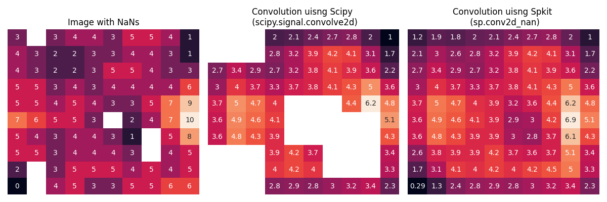
- 2D
sp.conv2d_nan
import numpy as np
import matplotlib.pyplot as plt
import seaborn as sns
import scipy
import spkit as sp
seed = 2
I = (sp.create_signal_2d(n=10,seed=seed,sg_winlen=3)*10).round(0)
np.random.seed(seed)
r = np.random.rand(*I.shape)
np.random.seed(None)
I[r<0.05] = np.nan
kernel = np.ones([3,3])/9
I_scipy = scipy.signal.convolve2d(I.copy(), kernel,mode='same', boundary='fill',fillvalue=0)
I_spkit = sp.conv2d_nan(I.copy(), kernel, boundary='fill',fillvalue=0)
plt.figure(figsize=(12,4))
plt.subplot(131)
sns.heatmap(I, annot=True,cbar=False,xticklabels='', yticklabels='')
plt.title('Image with NaNs')
plt.subplot(132)
sns.heatmap(I_scipy, annot=True,cbar=False,xticklabels='', yticklabels='')
plt.title('Convolution uisng Scipy \n (scipy.signal.convolve2d)')
plt.subplot(133)
sns.heatmap(I_spkit, annot=True,cbar=False,xticklabels='', yticklabels='')
plt.title('Convolution uisng Spkit \n (sp.conv2d_nan)')
plt.tight_layout()
plt.show()
Filling Missing values with inter/exterpolation
# 1D
# ~~~~~
#sp.fill_nans_1d
import numpy as np
import spkit as sp
x = np.array([1,1,np.nan, 3,4,9,3, np.nan])
y = sp.fill_nans_1d(x)
print(x)
print(y)
[ 1.  1. nan  3.  4.  9.  3. nan]
[ 1.  1.  2.  3.  4.  9.  3. -3.]
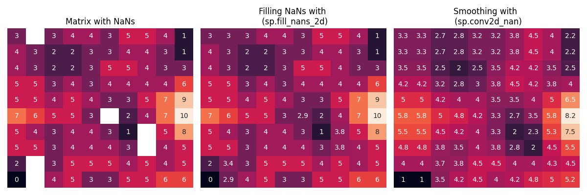
- 2D
sp.fill_nans_2d
import numpy as np
import matplotlib.pyplot as plt
import seaborn as sns
import scipy
import spkit as sp
seed = 2
I = (sp.create_signal_2d(n=10,seed=seed,sg_winlen=3)*10).round(0)
np.random.seed(seed)
r = np.random.rand(*I.shape)
I[r<0.05] = np.nan
np.random.seed(None)
kernel = np.ones([2,2])/4
I_spkit = sp.conv2d_nan(I.copy(), kernel, boundary='reflect',fillvalue=0)
I_fill, I_sm  = sp.fill_nans_2d(I.copy())
plt.figure(figsize=(12,4))
plt.subplot(131)
sns.heatmap(I, annot=True,cbar=False,xticklabels='', yticklabels='')
plt.title('Matrix with NaNs')
plt.subplot(132)
sns.heatmap(I_fill, annot=True,cbar=False,xticklabels='', yticklabels='')
plt.title('Filling NaNs with \n (sp.fill_nans_2d)')
plt.subplot(133)
sns.heatmap(I_spkit, annot=True,cbar=False,xticklabels='', yticklabels='')
plt.title('Smoothing with \n (sp.conv2d_nan)')
plt.tight_layout()
plt.show()
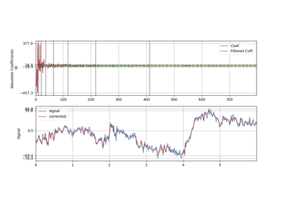
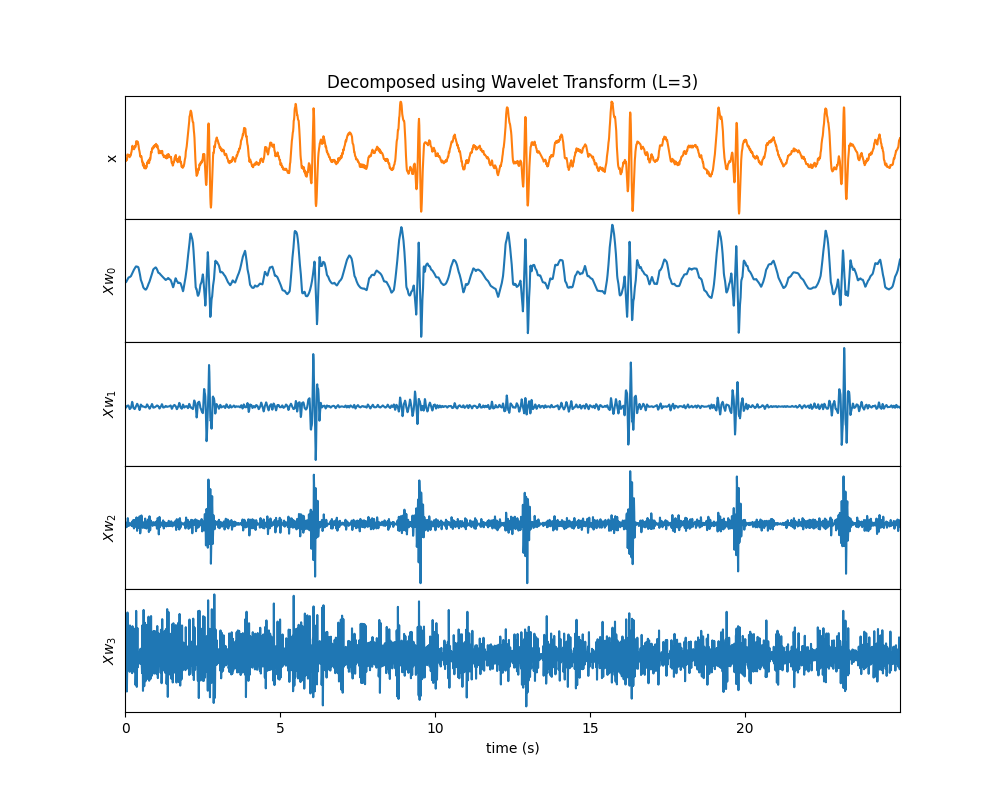
Wavelet Decomped Signals
Wavelet Transform
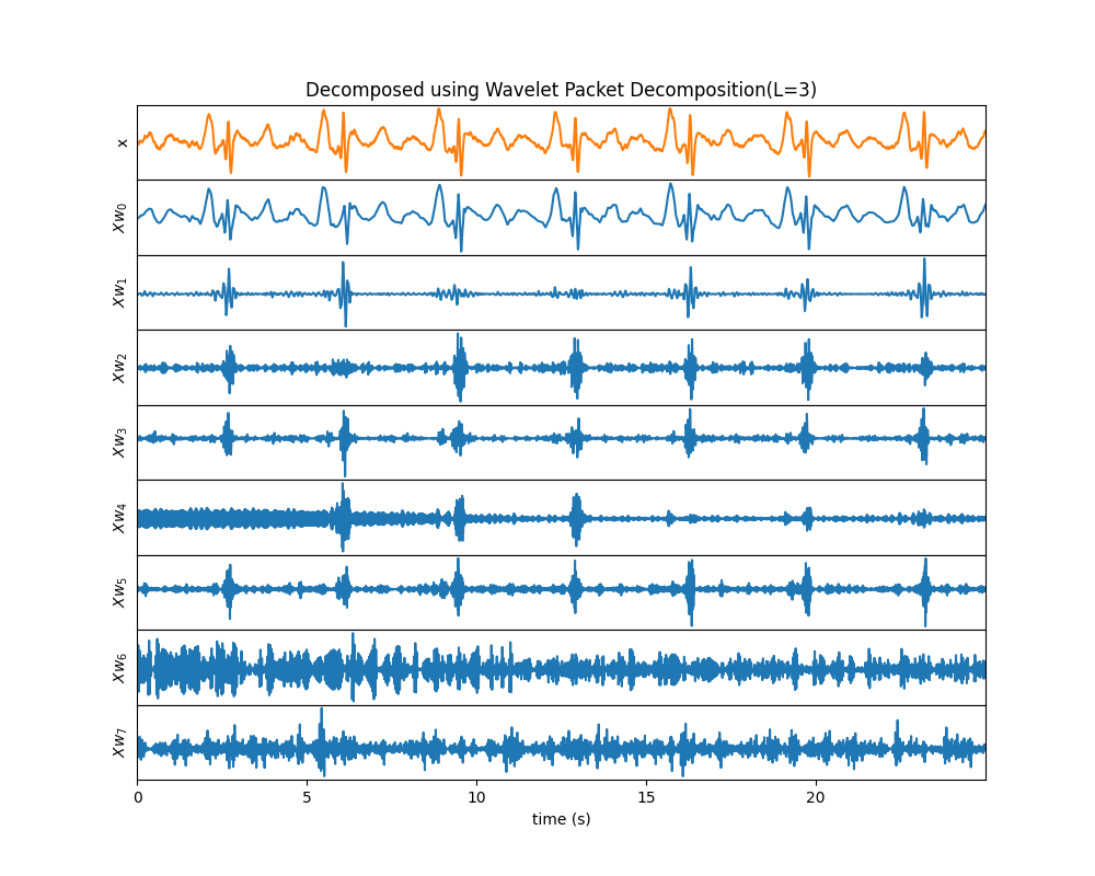
Wavelet Packet Decompositon
# Example 1: Wavelet Transform
# ~~~~~~~~~~~~~~~~~~~~~~~~~~~~~~
#
# sp.wavelet_decomposed_signals
import numpy as np
import matplotlib.pyplot as plt
import spkit as sp
x,fs,lead_names = sp.data.ecg_sample_12leads(sample=2)
x = x[:int(fs*5),5]
x = sp.filterDC_sGolay(x, window_length=fs//3+1)
t = np.arange(len(x))/fs
XR = sp.wavelet_decomposed_signals(x,wv='db3',L=3,plot_each=False,WPD=False)
plt.show()
Example 2: Wavelet Packet Decomposition
import numpy as np
import matplotlib.pyplot as plt
import spkit as sp
x,fs,lead_names = sp.data.ecg_sample_12leads(sample=2)
x = x[:int(fs*5),5]
x = sp.filterDC_sGolay(x, window_length=fs//3+1)
t = np.arange(len(x))/fs
XR = sp.wavelet_decomposed_signals(x,wv='db3',L=3,plot_each=False,WPD=True)
plt.show()
MEA: Multi-Electrode Array Processing
A full Documentation of MEA Processing Library is added.
MEA: Multi-Electrode Array Processing
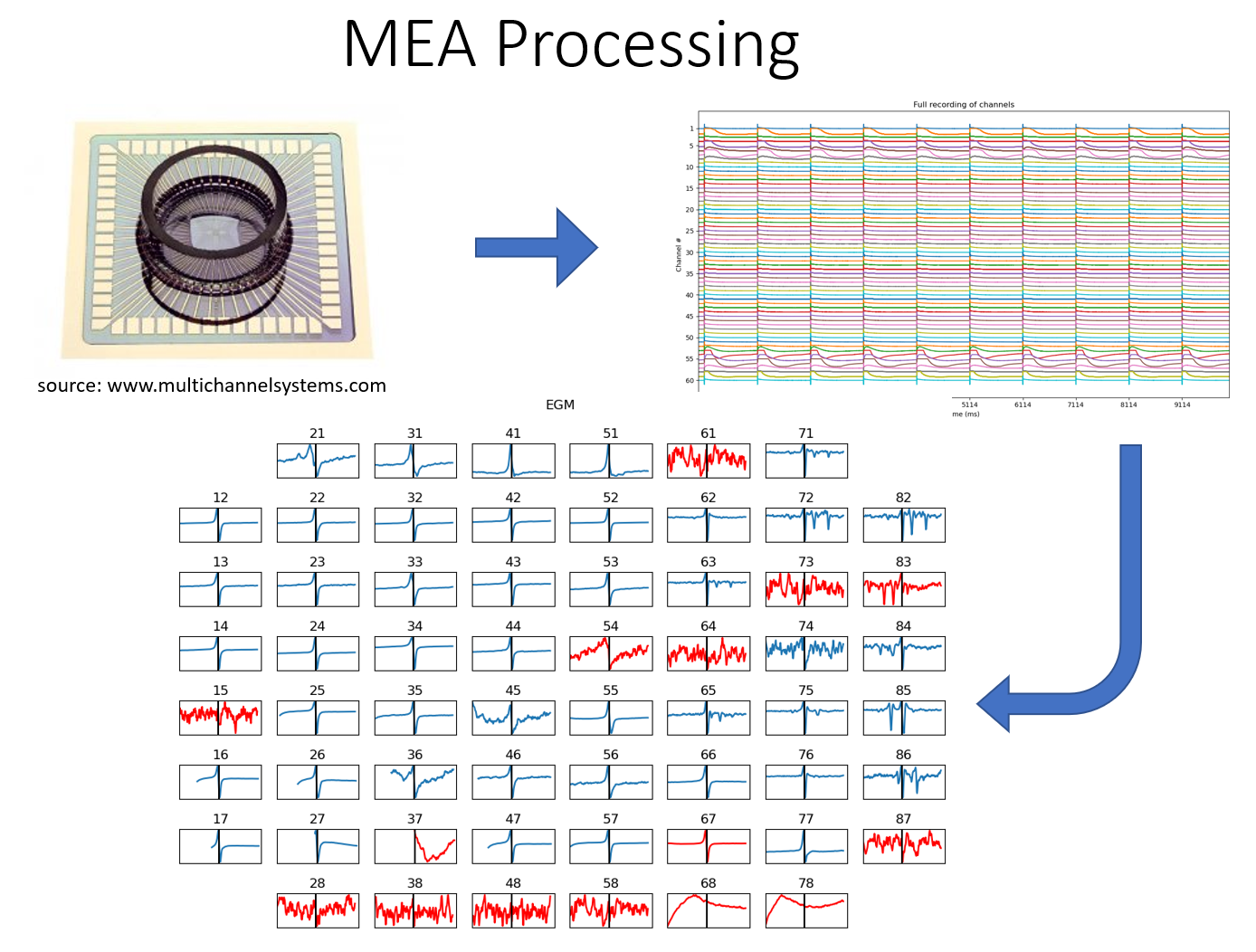
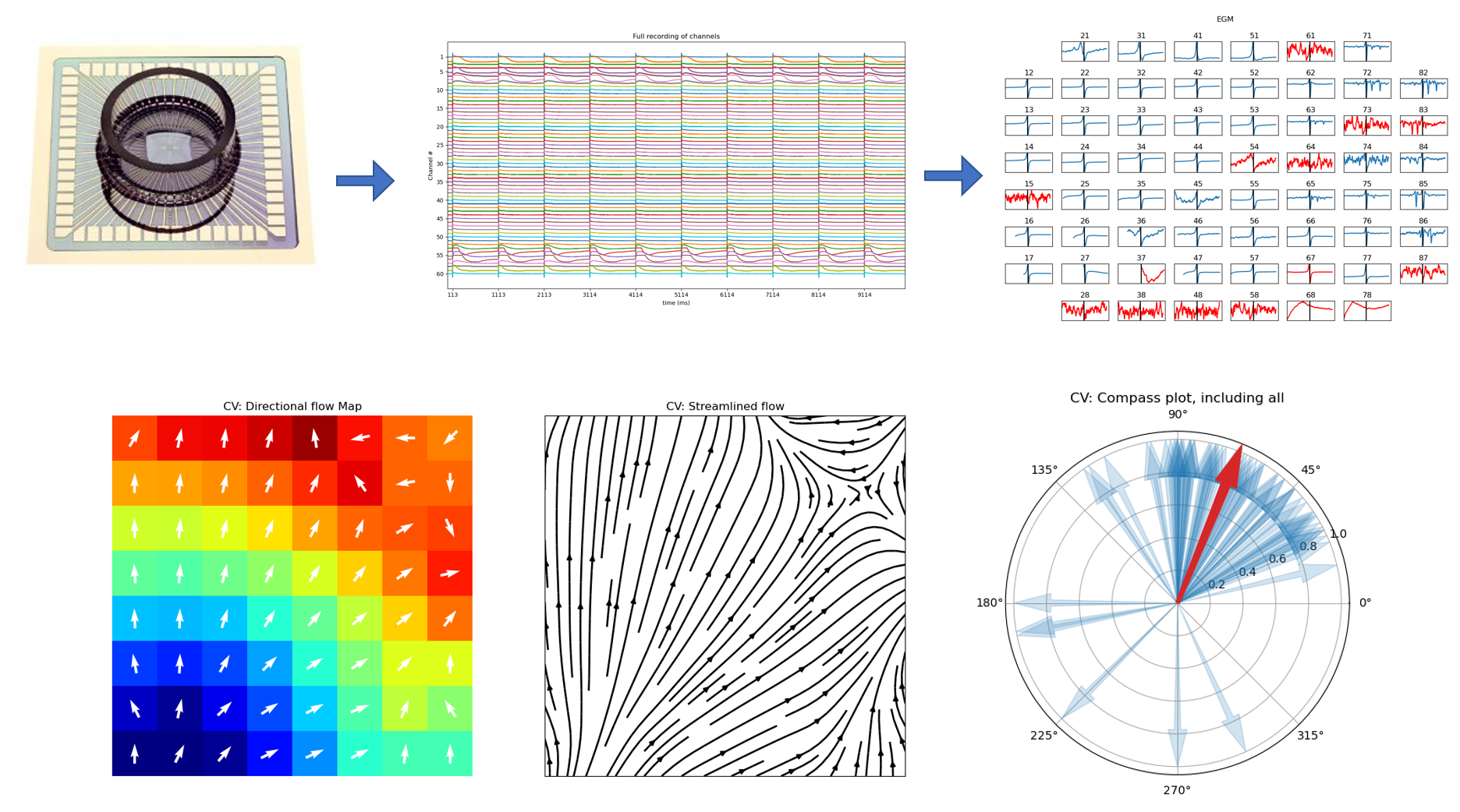
Check Examples of MEA
Total running time of the script: (0 minutes 1.395 seconds)
Related examples