Note
Go to the end to download the full example code or to run this example in your browser via JupyterLite or Binder
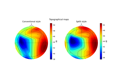
EEG Topographic Map
import numpy as np
import matplotlib.pyplot as plt
#from spkit import ICA
import spkit as sp
print('spkit version :', sp.__version__)
spkit version : 0.0.9.7
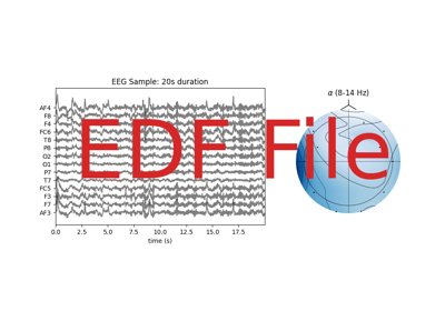
Load and filter EEG Signal
# Load sample EEG Data ( 16 sec, 128 smapling rate, 14 channel)
# Filter signal (with IIR highpass 0.5Hz)

X, fs, ch_names = sp.data.eeg_sample_14ch()


Xf = sp.filter_X(X.copy(),fs=128.0, band=[0.5], btype='highpass',ftype='SOS')

XR = sp.eeg.ATAR(Xf.copy(),wv='db3', winsize=128, thr_method='ipr',beta=0.2, k1=10, k2=100,OptMode='elim')
Rhythmic Powers,
# Total

Pm = sp.eeg.rhythmic_powers(X=XR.copy(),fs=fs,fBands=[[8,14], [15,32]],Sum=True,Mean=False,SD =True)[0]
Pm = 20*np.log10(Pm)

# in windows

Pmt = sp.eeg.rhythmic_powers_win(X=XR.copy(),winsize=128*2,overlap=64,fs=fs,
                                 fBands=[[8,14], [15,32]],Sum=True,Mean=False,SD =True)[0]
Pmt = 20*np.log10(Pmt)
Topomap of Total power
fig,ax = plt.subplots(1,2,figsize=(10,4))
Z1,im1 = sp.eeg.topomap(data=Pm[0],ch_names=ch_names,shownames=False,axes=ax[0],return_im=True)
Z2,im2 =sp.eeg.topomap(data=Pm[1],ch_names=ch_names,shownames=False,axes=ax[1],return_im=True)

ax[0].set_title(r'$\alpha$ : [8-14] Hz')
ax[1].set_title(r'$\beta$ : [15-32] Hz')
plt.colorbar(im1, ax=ax[0],label='dB')
plt.colorbar(im2, ax=ax[1],label='dB')
plt.suptitle('Spkit-style')
plt.show()

fig,ax = plt.subplots(1,2,figsize=(10,4))
Z1,im1 = sp.eeg.topomap(data=Pm[0],ch_names=ch_names,shownames=False,axes=ax[0],return_im=True,style='eeglab-mne')
Z2,im2 =sp.eeg.topomap(data=Pm[1],ch_names=ch_names,shownames=False,axes=ax[1],return_im=True,style='eeglab-mne')

ax[0].set_title(r'$\alpha$ : [8-14] Hz')
ax[1].set_title(r'$\beta$ : [15-32] Hz')
plt.colorbar(im1, ax=ax[0],label='dB')
plt.colorbar(im2, ax=ax[1],label='dB')
plt.suptitle('eeglab/mne-style')
plt.show()
![Spkit-style, $\alpha$ : [8-14] Hz, $\beta$ : [15-32] Hz](../../_images/sphx_glr_plot_sp_eeg_topomaps_001.png)
![eeglab/mne-style, $\alpha$ : [8-14] Hz, $\beta$ : [15-32] Hz](../../_images/sphx_glr_plot_sp_eeg_topomaps_002.png)
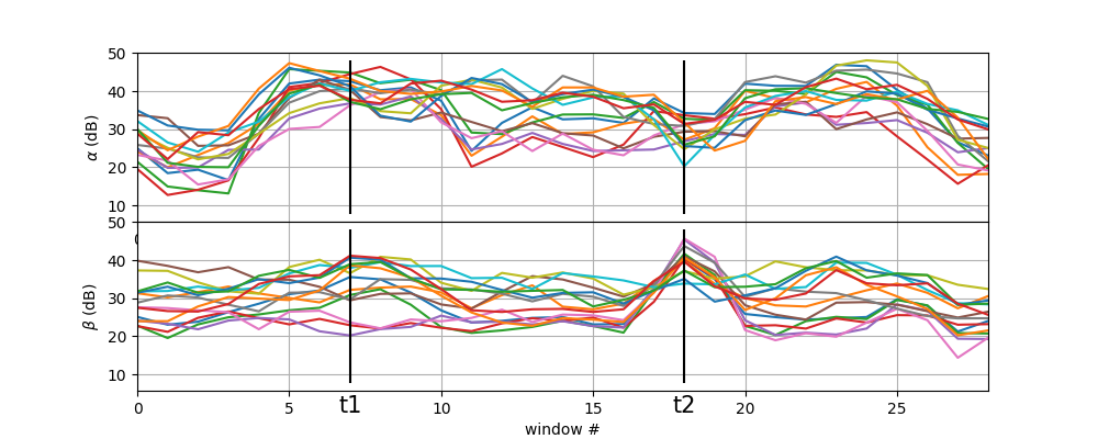
Topomap for specific time-windows
t1,t2 = 7,18

plt.figure(figsize=(10,4))
plt.subplot(211)
plt.plot(Pmt[:,0,:])
plt.xlim([0,Pmt.shape[0]-1])
plt.vlines([t1,t2],ymin=Pmt[:,0,:].min()-5,ymax=Pmt[:,0,:].max(),color='k')
plt.grid()
plt.ylabel(r'$\alpha$ (dB)')
plt.subplot(212)
plt.plot(Pmt[:,1,:])
plt.xlim([0,Pmt.shape[0]-1])
plt.vlines([t1,t2],ymin=Pmt[:,0,:].min()-5,ymax=Pmt[:,0,:].max(),color='k')
plt.grid()
plt.ylabel(r'$\beta$ (dB)')
plt.xlabel('window #')
plt.text(t1,0,'t1',fontsize=15,ha='center')
plt.text(t2,0,'t2',fontsize=15,ha='center')
plt.subplots_adjust(hspace=0)
plt.show()

fig,ax = plt.subplots(1,2,figsize=(10,4))
Z1,im1 = sp.eeg.topomap(data=Pmt[t1,0,:],ch_names=ch_names,vmin=Pmt[t1].min(),vmax=Pmt[t1].max(),
                        shownames=False,axes=ax[0],return_im=True)
Z2,im2 =sp.eeg.topomap(data=Pmt[t1,1,:],ch_names=ch_names,vmin=Pmt[t1].min(),vmax=Pmt[t1].max(),
                       shownames=False,axes=ax[1],return_im=True)

ax[0].set_title(r'$\alpha$ : [8-14] Hz')
ax[1].set_title(r'$\beta$ : [15-32] Hz')
#plt.colorbar(im1, ax=ax[0],label='dB')
plt.colorbar(im2, ax=ax[1],label='dB')
plt.suptitle('t1')
plt.show()

fig,ax = plt.subplots(1,2,figsize=(10,4))
Z1,im1 = sp.eeg.topomap(data=Pmt[t2,0,:],ch_names=ch_names,vmin=Pmt[t2].min(),vmax=Pmt[t2].max(),
                        shownames=False,axes=ax[0],return_im=True)
Z2,im2 =sp.eeg.topomap(data=Pmt[t2,1,:],ch_names=ch_names,vmin=Pmt[t2].min(),vmax=Pmt[t2].max(),
                       shownames=False,axes=ax[1],return_im=True)

ax[0].set_title(r'$\alpha$ : [8-14] Hz')
ax[1].set_title(r'$\beta$ : [15-32] Hz')
#plt.colorbar(im1, ax=ax[0],label='dB')
plt.colorbar(im2, ax=ax[1],label='dB')
plt.suptitle('t2')
plt.show()
![t1, $\alpha$ : [8-14] Hz, $\beta$ : [15-32] Hz](../../_images/sphx_glr_plot_sp_eeg_topomaps_004.png)
![t2, $\alpha$ : [8-14] Hz, $\beta$ : [15-32] Hz](../../_images/sphx_glr_plot_sp_eeg_topomaps_005.png)
Total running time of the script: (0 minutes 0.829 seconds)
Related examples
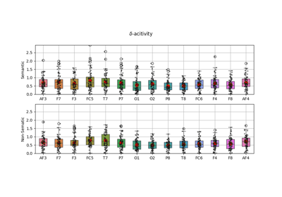
EEG Computing Rhythmic Features - PhyAAt - Semanticity
EEG Computing Rhythmic Features - PhyAAt - Semanticity