Note

Go to the end to download the full example code or to run this example in your browser via JupyterLite or Binder

EEG Computing Rhythmic Features - PhyAAt - Semanticity¶

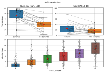
In this example, we are using PhyAAt Dataset to show the how to compute rhythmic features and compare them.

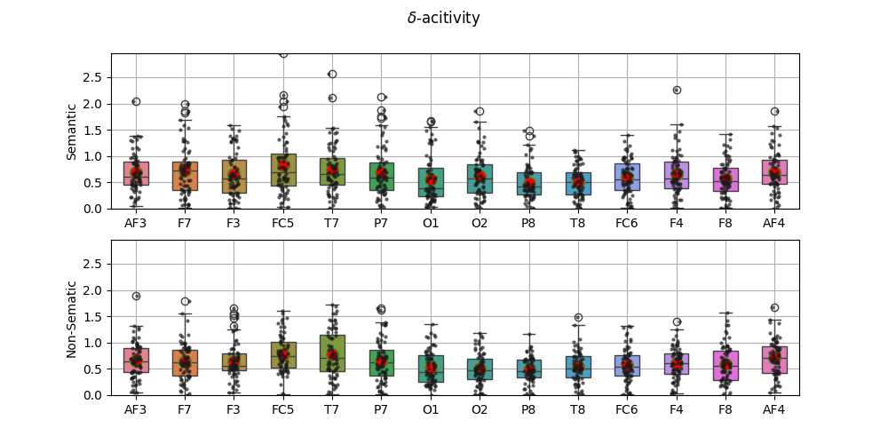
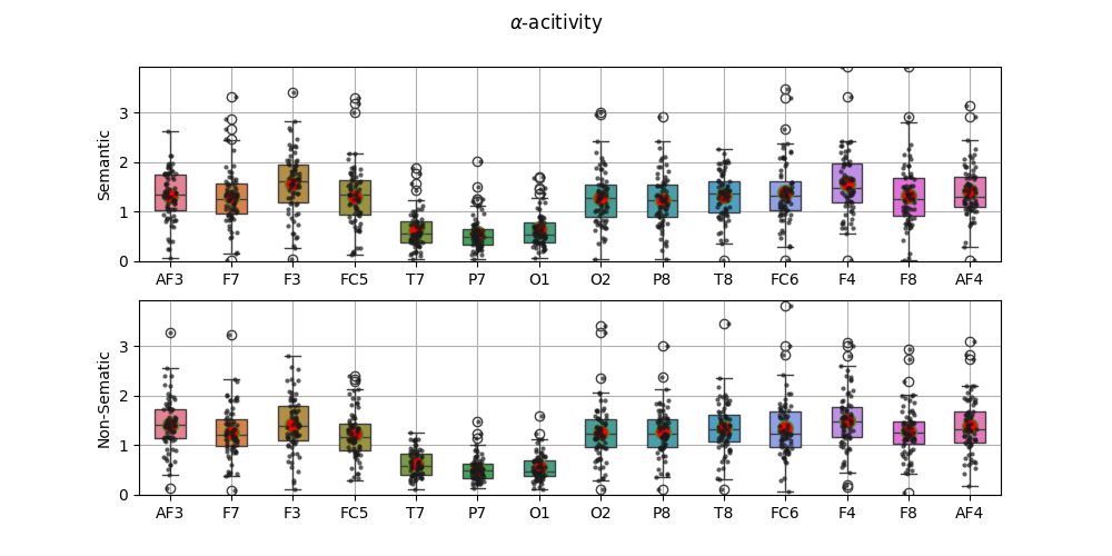
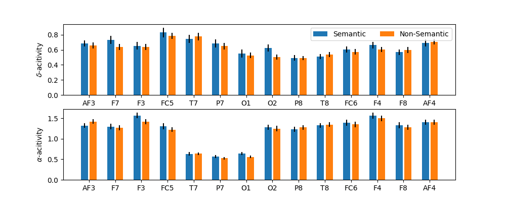
In this example, we compute average power in Delta frequency Band (0.5-4) Hz and Alpha frequency band (8-14) Hz. We compare the power in each eletrode for semantic and non-semantic stimuli.

import numpy as np
import matplotlib.pyplot as plt
import spkit as sp
print('spkit version :', sp.__version__)

spkit version : 0.0.9.7

PhyAAt Dataset¶

import phyaat as ph


# download subject 10 data

dirPath = ph.download_data(baseDir='../PhyAAt/data/', subject=10,verbose=0,overwrite=False)
SubID = ph.ReadFilesPath(dirPath)
Subj = ph.Subject(SubID[10])

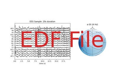
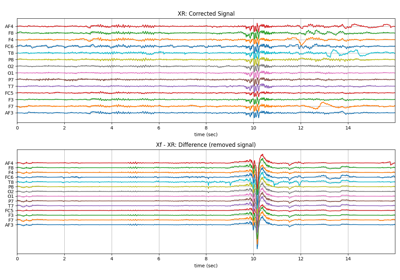
# filter and remove artifacts
Subj.filter_EEG(band =[0.5],btype='highpass',method='SOS',order=5)
Subj.correct(method='ATAR',verbose=1,winsize=128,
            wv='db3',thr_method='ipr',IPR=[25,75],beta=0.1,k1=10,k2 =100,est_wmax=100,
            OptMode ='elim',fs=128.0,use_joblib=False)

# Extract EEG of listening segments
L,_,_, _, Cols = Subj.getLWR()
fs=128

# label of semanticity
Sem = np.array([L[i][32][-3] for i in range(len(L))])

idx0 = np.where(Sem==0)[0]  # semantic
idx1 = np.where(Sem==1)[0]  # non-semantic

ch_names = Cols[1:15]

E0 = [L[i][:,1:15].astype(float) for i in idx0] # semantic
E1 = [L[i][:,1:15].astype(float) for i in idx1] # non-semantic

Total Subjects :  1

# Listening Segmnts :  144
# Writing Segmnts   :  144
# Resting Segmnts   :  144
# Scores :  144

Extract Rhythmic Features¶

XF0 = []
for X in E0:
    _,Pm,_ = sp.eeg.rhythmic_powers(X=X.copy(),fs=fs,fBands=[[4],[8,14]],Sum=False,Mean=True,SD =False)
    XF0.append(Pm)

XF1 = []
for X in E1:
    _,Pm,_ = sp.eeg.rhythmic_powers(X=X.copy(),fs=fs,fBands=[[4],[8,14]],Sum=False,Mean=True,SD =False)
    XF1.append(Pm)

XF0 = np.array(XF0)
XF1 = np.array(XF1)

Plots to compare¶

m1 = np.max([XF0[:,0,:].max(), XF1[:,0,:].max()])
m2 = np.max([XF0[:,1,:].max(), XF1[:,1,:].max()])

fig,ax = plt.subplots(2,1,figsize=(10,5))
sp.stats.plot_groups_boxes(XF0[:,0,:],ax=ax[0],ylab='Semantic',xlabels=ch_names,
                           strip_kw=dict(color="0.1",alpha=0.7,size=3))
sp.stats.plot_groups_boxes(XF1[:,0,:],ax=ax[1],ylab='Non-Sematic',xlabels=ch_names,
                           strip_kw=dict(color="0.1",alpha=0.7,size=3))
ax[0].set_ylim([0,m1])
ax[1].set_ylim([0,m1])
fig.suptitle(r'$\delta$-acitivity')
plt.show()


fig,ax = plt.subplots(2,1,figsize=(10,5))
sp.stats.plot_groups_boxes(XF0[:,1,:],ax=ax[0],ylab='Semantic',xlabels=ch_names,
                           strip_kw=dict(color="0.1",alpha=0.7,size=3))
sp.stats.plot_groups_boxes(XF1[:,1,:],ax=ax[1],ylab='Non-Sematic',xlabels=ch_names,
                           strip_kw=dict(color="0.1",alpha=0.7,size=3))
ax[0].set_ylim([0,m2])
ax[1].set_ylim([0,m2])
fig.suptitle(r'$\alpha$-acitivity')
plt.show()

t = np.arange(14)*3
plt.figure(figsize=(10,4))
plt.subplot(211)
plt.bar(t,XF0[:,0,:].mean(0),yerr=XF0[:,0,:].std(0)/np.sqrt(77-1),label='Semantic')
plt.bar(t+1,XF1[:,0,:].mean(0),yerr=XF1[:,0,:].std(0)/np.sqrt(77-1),label='Non-Semantic')
plt.xticks(t+0.5,ch_names)
plt.legend(loc=1,ncol=2)
plt.ylabel(r'$\delta$-acitivity')

plt.subplot(212)
plt.bar(t,XF0[:,1,:].mean(0),yerr=XF0[:,1,:].std(0)/np.sqrt(77-1),label='Semantic')
plt.bar(t+1,XF1[:,1,:].mean(0),yerr=XF1[:,1,:].std(0)/np.sqrt(77-1),label='Non-Semantic')
plt.xticks(t+0.5,ch_names)
plt.ylabel(r'$\alpha$-acitivity')
plt.show()