Note
Go to the end to download the full example code or to run this example in your browser via JupyterLite or Binder
Sample and Approximate Entropy: Comparison
In this example, we compare Approximate Emtropy with Sample Entropy
![x1~$\mathcal{Sin}$, x2~$\mathcal{N}(0,1)$, x3~$\mathcal{U}[-0.5,0.5]$](../../_images/sphx_glr_plot_it_sample_approx_entropy_comp_001.png)
0.23429427895105137 0.5921334630488566 0.6720444345470105
0.23462714901066314 2.1931512519485836 2.24992380933707
------------------------------------------------------------
         Aproximate Entropy      Sample Entropy
------------------------------------------------------------
x1:      0.23429427895105137     0.23462714901066314
x2:      0.5921334630488566      2.1931512519485836
x3:      0.6720444345470105      2.24992380933707
------------------------------------------------------------
------------------------------------------------------------
-          time:         Mean            SD
------------------------------------------------------------
Approx Entropy:  1.0331743999999958      0.011493672547972069
Sample Entropy:  0.04396960000000263     9.239610381009533e-05
------------------------------------------------------------

  4%|▓▓                                                |21\1|
  9%|▓▓▓▓                                              |21\2|
 14%|▓▓▓▓▓▓▓                                           |21\3|
 19%|▓▓▓▓▓▓▓▓▓                                         |21\4|
 23%|▓▓▓▓▓▓▓▓▓▓▓                                       |21\5|
 28%|▓▓▓▓▓▓▓▓▓▓▓▓▓▓                                    |21\6|
 33%|▓▓▓▓▓▓▓▓▓▓▓▓▓▓▓▓                                  |21\7|
 38%|▓▓▓▓▓▓▓▓▓▓▓▓▓▓▓▓▓▓▓                               |21\8|
 42%|▓▓▓▓▓▓▓▓▓▓▓▓▓▓▓▓▓▓▓▓▓                             |21\9|
 47%|▓▓▓▓▓▓▓▓▓▓▓▓▓▓▓▓▓▓▓▓▓▓▓                           |21\10|
 52%|▓▓▓▓▓▓▓▓▓▓▓▓▓▓▓▓▓▓▓▓▓▓▓▓▓▓                        |21\11|
 57%|▓▓▓▓▓▓▓▓▓▓▓▓▓▓▓▓▓▓▓▓▓▓▓▓▓▓▓▓                      |21\12|
 61%|▓▓▓▓▓▓▓▓▓▓▓▓▓▓▓▓▓▓▓▓▓▓▓▓▓▓▓▓▓▓                    |21\13|
 66%|▓▓▓▓▓▓▓▓▓▓▓▓▓▓▓▓▓▓▓▓▓▓▓▓▓▓▓▓▓▓▓▓▓                 |21\14|
 71%|▓▓▓▓▓▓▓▓▓▓▓▓▓▓▓▓▓▓▓▓▓▓▓▓▓▓▓▓▓▓▓▓▓▓▓               |21\15|
 76%|▓▓▓▓▓▓▓▓▓▓▓▓▓▓▓▓▓▓▓▓▓▓▓▓▓▓▓▓▓▓▓▓▓▓▓▓▓▓            |21\16|
 80%|▓▓▓▓▓▓▓▓▓▓▓▓▓▓▓▓▓▓▓▓▓▓▓▓▓▓▓▓▓▓▓▓▓▓▓▓▓▓▓▓          |21\17|
 85%|▓▓▓▓▓▓▓▓▓▓▓▓▓▓▓▓▓▓▓▓▓▓▓▓▓▓▓▓▓▓▓▓▓▓▓▓▓▓▓▓▓▓        |21\18|
 90%|▓▓▓▓▓▓▓▓▓▓▓▓▓▓▓▓▓▓▓▓▓▓▓▓▓▓▓▓▓▓▓▓▓▓▓▓▓▓▓▓▓▓▓▓▓     |21\19|
 95%|▓▓▓▓▓▓▓▓▓▓▓▓▓▓▓▓▓▓▓▓▓▓▓▓▓▓▓▓▓▓▓▓▓▓▓▓▓▓▓▓▓▓▓▓▓▓▓   |21\20|
100%|▓▓▓▓▓▓▓▓▓▓▓▓▓▓▓▓▓▓▓▓▓▓▓▓▓▓▓▓▓▓▓▓▓▓▓▓▓▓▓▓▓▓▓▓▓▓▓▓▓▓|21\21|
Done!
import numpy as np
import matplotlib.pyplot as plt
import spkit as sp
fs = 1000
t = np.arange(1000)/fs
x1 = np.cos(2*np.pi*10*t)+np.cos(2*np.pi*30*t)+np.cos(2*np.pi*20*t)
np.random.seed(1)
x2 = np.random.randn(1000)
x3 = np.random.rand(1000)-0.5
plt.figure(figsize=(12,3))
plt.subplot(131)
plt.plot(t,x1)
plt.title(r'x1~$\mathcal{Sin}$')
plt.subplot(132)
plt.plot(t,x2)
plt.title(r'x2~$\mathcal{N}(0,1)$')
plt.subplot(133)
plt.plot(t,x3)
plt.title(r'x3~$\mathcal{U}[-0.5,0.5]$')
plt.tight_layout()
plt.show()
Hx1_apx = sp.entropy_approx(x1,m=3,r=0.2*np.std(x1))
Hx2_apx = sp.entropy_approx(x2,m=3,r=0.2*np.std(x2))
Hx3_apx = sp.entropy_approx(x3,m=3,r=0.2*np.std(x3))
print(Hx1_apx, Hx2_apx, Hx3_apx)
Hx1_sae = sp.entropy_sample(x1,m=3,r=0.2*np.std(x1))
Hx2_sae = sp.entropy_sample(x2,m=3,r=0.2*np.std(x2))
Hx3_sae = sp.entropy_sample(x3,m=3,r=0.2*np.std(x3))
print(Hx1_sae, Hx2_sae, Hx3_sae)
print('--'*30)
print(' \t Aproximate Entropy \t Sample Entropy')
print('--'*30)
print(f'x1:\t {Hx1_apx} \t {Hx1_sae}')
print(f'x2:\t {Hx2_apx} \t {Hx2_sae}')
print(f'x3:\t {Hx3_apx} \t {Hx3_sae}')
print('--'*30)
import time
tt1 = []
for _ in range(5):
start = time.process_time()
sp.entropy_approx(x1,m=3,r=0.2*np.std(x1))
tt1.append(time.process_time() - start)
#print(time.process_time() - start)
tt2 = []
for _ in range(5):
start = time.process_time()
sp.entropy_sample(x1,m=3,r=0.2*np.std(x1))
tt2.append(time.process_time() - start)
#print(time.process_time() - start)
print('--'*30)
print('- time: \t Mean \t SD')
print('--'*30)
print(f'Approx Entropy:\t {np.mean(tt1)} \t {np.std(tt1)}')
print(f'Sample Entropy:\t {np.mean(tt2)} \t {np.std(tt2)}')
print('--'*30)
ApSmEn1 = []
ApSmEn2 = []
SD = []
Ps = np.arange(0,1+0.04,0.05)
for i,p in enumerate(Ps):
sp.utils.ProgBar_JL(i,len(Ps))
x41 = x1*(1-p) + p*x2
aprEn = sp.entropy_approx(x41,m=3,r=0.2*np.std(x41))
smEn = sp.entropy_sample(x41,m=3,r=0.2*np.std(x41))
ApSmEn1.append([p,aprEn,smEn])
x42 = x1*(1-p) + p*x3
aprEn = sp.entropy_approx(x42,m=3,r=0.2*np.std(x42))
smEn = sp.entropy_sample(x42,m=3,r=0.2*np.std(x42))
ApSmEn2.append([p,aprEn,smEn])
SD.append([p,0.2*np.std(x41),0.2*np.std(x42)])
ApSmEn1 = np.array(ApSmEn1)
ApSmEn2 = np.array(ApSmEn2)
SD = np.array(SD)
plt.figure(figsize=(11,5))
plt.subplot(121)
plt.plot(ApSmEn1[:,0],ApSmEn1[:,1:], label=['ApproxEn', 'SamEn'])
plt.xlim([0,1])
plt.xlabel('p')
plt.ylabel('SamEn/AproxEn')
plt.grid()
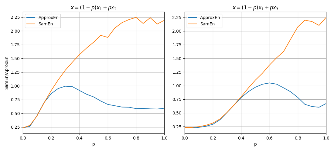
plt.title(r'$x = (1-p)x_1 + px_2$')
plt.legend()
plt.subplot(122)
plt.plot(ApSmEn2[:,0],ApSmEn2[:,1:], label=['ApproxEn', 'SamEn'])
plt.xlim([0,1])
plt.xlabel('p')
plt.legend()
plt.grid()
plt.title(r'$x = (1-p)x_1 + px_3$')
plt.tight_layout()
plt.show()
Total running time of the script: (0 minutes 53.832 seconds)
Related examples
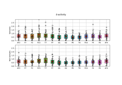
EEG Computing Rhythmic Features - PhyAAt - Semanticity
EEG Computing Rhythmic Features - PhyAAt - Semanticity