spkit.eeg.topomap

spkit.eeg.topomap(data, pos=None, ch_names=None, res=64, Zi=None, show=True, return_im=False, standard='1020', style='spkit', **kwargs)

Display Topographical Map of EEG, with given values

Parameters:

data: 1d-array

• 1d-array of values for the each electrode.

pos: 2d-array, deafult=None

• 2D projection points for each electroed

• computed using one of either s1020_get_epos2d, s1010_get_epos2d, s1005_get_epos2d

  or provided by custom system

• MUST BE same number of points as data points, e.g. pos.shape[0]==data.shape[0]

• IF None, then computed using ch_names system style provided.

ch_names: list of str, default=None

• name of the channels/electrodes

• should be same size as data.shape[0]

• IF pos is None, this is used to compute projection points (pos), in that case, make sure to provide valid channel names and respective system. or compute using s1020_get_epos2d, s1010_get_epos2d, s1005_get_epos2d

• This list is also used to shownames of sensors, if shownames is True.

Note

IMPORTANT Either pos or valid ch_names should be provided

res: int, default=64

• resolution of image to be generated, (res,res)

Zi: 2d-array, default None,

• Pre-computed Image of topographic map.

• if provided, then data is ignored, else image is generated using data-points

show: bool, defult=True

• if False, then plot is not produced

• useful, when interested in only generating Zi images

return_im: bool, default=False

• if True, in addtion to Zi (generate Image), im object is also returned

standard: str, default =’1020’

• it is used ONLY if pos is None

• standard to extract pos from ch_names

• check s1020_get_epos2d, s1010_get_epos2d, s1005_get_epos2d

style: str, default = ‘spkit’

• it is used ONLY if pos is None and standard is ‘1020’

• style to extract pos from ch_names

• check s1020_get_epos2d

kwargs:

There are other arguments which can be supplied to modify the topomap disply

• warn: bool, default True

  • set it to False, to supress the warnings of change names

• c:scalar,default=0.5

  • shifting origin, only used if shift_origin is True

• s:scalar,default=0.85

  • scale the electrod postions by the factor s, higher it is more spreaded they are

• (fx, fy):scalar,default=(0.5, 0.5)

  • x-lim, y-lim of grid,

• (rx,ry):scalar,default=(1,1)

  • radius of the ellips to clip, higher it is more outter area is covered

• shift_origin=False

  • If True, center point of electrode poisition will be the origin = (0,0)

  • it uses c parameter to shift the origin

  • pos -= c*([dx, dy])

  • if c=1, new origin will be at 0,0

• axes=None: Axes to use for plotting, if None, then created using plt.gca()

• For Image display, plt.imshow kwargs:

  • (cmap=’jet’,origin=’lower’,aspect=’equal’,vmin=None,vmax=None,interpolation=None)

• contours=True: contour lines

  • if True, contours_n contours are shown with linewidth of contours_lw

• showsensors=True: sensor location

  • display sensors/eletrodes as dots

  • add cicles of sensors using sensor_prop

• shownames=True

  • if True, show them, using fontdict and font_prop

  • default fontdict=None, font_prop=dict()

• showhead=True

  • If True, show head, using head_prop (default head_prop =dict(markersize=30))

  • it is passed to ax.plot as kwargs

• showbound=True: show boundary

  • uses bound_prop=dict(rx=0.85,ry=0.85,xy=(0,0),color=’k’,alpha=0.5)

  • could be used to show oval shape head, with rx,ry = 0.85,0.9

• show_vhlines=True: lines

  • show verticle and horizontal lines passing through origin

• show_colorbar=False, colorbar

  • if True, show colorbar with label as colorbar_label

• match_shed=True: boundary

  • if True, center of boundary is same as center of grid.

Returns:

Zi: 2d-array

• 2D full Grid as image, without circular crop.

• Obatained from Inter/exterpolation

im: image object

• returned from im = ax.imshow()

• only of return_im is True

See also

Gen_SSFI

Examples

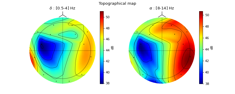
#sp.eeg.topomap
import numpy as np
import matplotlib.pyplot as plt
import spkit as sp
X,fs, ch_names = sp.data.eeg_sample_14ch()
X = sp.filterDC_sGolay(X, window_length=fs//3+1)
Px,Pm,Pd = sp.eeg.rhythmic_powers(X=X,fs=fs,fBands=[[4],[8,14]],Sum=True,Mean=True,SD =True)
Px = 20*np.log10(Px)
pos1, ch = sp.eeg.s1020_get_epos2d(ch_names,style='eeglab-mne')
pos2, ch = sp.eeg.s1020_get_epos2d(ch_names,style='spkit')
fig, ax = plt.subplots(1,2,figsize=(10,4))
Z1i,im1 = sp.eeg.topomap(pos=pos1,data=Px[0],axes=ax[0],return_im=True)
Z2i,im2 = sp.eeg.topomap(pos=pos1,data=Px[1],axes=ax[1],return_im=True)
ax[0].set_title(r'$\delta$ : [0.5-4] Hz')
ax[1].set_title(r'$\alpha$ : [8-14] Hz')
plt.colorbar(im1, ax=ax[0],label='dB')
plt.colorbar(im2, ax=ax[1],label='dB')
plt.suptitle('Topographical map')
plt.show()

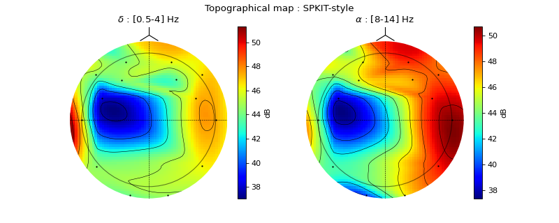
fig, ax = plt.subplots(1,2,figsize=(10,4))
Z1i,im1 = sp.eeg.topomap(pos=pos2,data=Px[0],axes=ax[0],return_im=True)
Z2i,im2 = sp.eeg.topomap(pos=pos2,data=Px[1],axes=ax[1],return_im=True)
ax[0].set_title(r'$\delta$ : [0.5-4] Hz')
ax[1].set_title(r'$\alpha$ : [8-14] Hz')
plt.colorbar(im1, ax=ax[0],label='dB')
plt.colorbar(im2, ax=ax[1],label='dB')
plt.suptitle('Topographical map : SPKIT-style')
plt.show()

Examples using spkit.eeg.topomap

EEG Data from EDF File

EEG Data from EDF File