spkit.dispersion_entropy
- spkit.dispersion_entropy(x, classes=10, scale=1, emb_dim=2, delay=1, mapping_type='cdf', de_normalize=False, A=100, Mu=100, return_all=False, warns=True)
Dispersion Entropy of signal \(H_{de}(X)\)
Calculate dispersion entropy of signal x (multiscale)
Dispersion Entropy
- Parameters:
- xinput signal x - 1d-array of shape=(n,)
- classes: number of classes - (levels of quantization of amplitude) (default=10)
- emb_dim: embedding dimension,
- delaytime delay (default=1)
- scaledownsampled signal with low resolution (default=1) - for multipscale dispersion entropy
- mapping_type: mapping method to discretizing signal (default=’cdf’)
: options = {‘cdf’,’a-law’,’mu-law’,’fd’}
- Afactor for A-Law- if mapping_type = ‘a-law’
- Mufactor for μ-Law- if mapping_type = ‘mu-law’
- de_normalize: (bool) if to normalize the entropy, to make it comparable with different signal with different
number of classes and embeding dimensions. default=0 (False) - no normalizations
- if de_normalize=1:
dispersion entropy is normalized by log(Npp); Npp=total possible patterns. This is classical way to normalize entropy since max{H(x)}<=np.log(N) for possible outcomes. However, in case of limited length of signal (sequence), it would be not be possible to get all the possible patterns and might be incorrect to normalize by log(Npp), when len(x)<Npp or len(x)<classes**emb_dim. For example, given signal x with discretized length of 2048 samples, if classes=10 and emb_dim=4, the number of possible patterns Npp = 10000, which can never be found in sequence length < 10000+4. To fix this, the alternative way to nomalize is recommended as follow.
select this when classes**emb_dim < (N-(emb_dim-1)*delay)
- de_normalize=2: (recommended for classes**emb_dim > len(x)/scale)
dispersion entropy is normalized by log(Npf); Npf [= (len(x)-(emb_dim - 1) * delay)] the total number of patterns founds in given sequence. This is much better normalizing factor. In worst case (lack of better word) - for a very random signal, all Npf patterns could be different and unique, achieving the maximum entropy and for a constant signal, all Npf will be same achieving to zero entropy
select this when classes**emb_dim > (N-(emb_dim-1)*delay)
- de_normalize=3:
dispersion entropy is normalized by log(Nup); number of total unique patterns (NOT RECOMMENDED) - it does not make sense (not to me, at least)
- de_normalize=4:
auto select normalizing factor
if classes**emb_dim > (N-(emb_dim-1)*delay), then de_normalize=2
if classes**emb_dim > (N-(emb_dim-1)*delay), then de_normalize=2
- Returns:
- disp_entrfloat
dispersion entropy of the signal
- probarray
probability distribution of patterns
- if return_all =True:
- patterns_dict: dict
dictionary of patterns and respective frequencies
- x_discretearray
discretized signal x
- (Npf,Npp,Nup): tuple of 3
Npf - total_patterns_found, Npp - total_patterns_possible
Nup - total unique patterns found
Npf number of total patterns in discretized signal (not total unique patterns)
See also
dispersion_entropy_multiscale_refinedDispersion Entropy multi-scale
entropyEntropy
entropy_sampleSample Entropy
entropy_approxApproximate Entropy
entropy_spectralSpectral Entropy
entropy_svdSVD Entropy
entropy_permutationPermutation Entropy
entropy_differentialDifferential Entropy
References
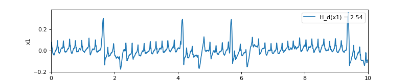
Examples
import numpy as np
import matplotlib.pyplot as plt
import spkit as sp
np.random.seed(1)
x1, fs = sp.data.optical_sample(sample=1)
t = np.arange(len(x1))/fs
H_de1, prob1  = sp.dispersion_entropy(x1,classes=10,scale=1)
print('DE of x1 = ',H_de1)
plt.figure(figsize=(10,2))
plt.plot(t,x1, label=f'H_d(x1) = {H_de1:,.2f}')
plt.xlim([t[0],t[-1]])
plt.ylabel('x1')
plt.xlabel('time (s)')
plt.legend(loc='upper right')
plt.show()