spkit.dispersion_entropy_multiscale_refined

spkit.dispersion_entropy_multiscale_refined(x, classes=10, scales=[1, 2, 3, 4, 5], emb_dim=2, delay=1, mapping_type='cdf', de_normalize=False, A=100, Mu=100, return_all=False, warns=True)

Multiscale refined Dispersion Entropy of signal \(H_{de}(X)\)

Calculate multiscale refined dispersion entropy of signal x

compute dispersion entropy at different scales (defined by argument - ‘scales’) and combining the patterns found at different scales to compute final dispersion entropy

Parameters:

xinput signal x - 1d-array of shape=(n,)

classesnumber of classes - (levels of quantization of amplitude) (default=10)

emb_dimembedding dimension,

delaytime delay (default=1)

scaleslist or 1d array of scales to be considered to refine the dispersion entropy

mapping_type: mapping method to discretizing signal (default=’cdf’)

: options = {‘cdf’,’a-law’,’mu-law’,’fd’}

Afactor for A-Law- if mapping_type = ‘a-law’

Mufactor for μ-Law- if mapping_type = ‘mu-law’

de_normalize: (bool) if to normalize the entropy, to make it comparable with different signal with different

number of classes and embeding dimensions. default=0 (False) - no normalizations

if de_normalize=1:

• dispersion entropy is normalized by log(Npp); Npp=total possible patterns. This is classical way to normalize entropy since max{H(x)}<=np.log(N) for possible outcomes. However, in case of limited length of signal (sequence), it would be not be possible to get all the possible patterns and might be incorrect to normalize by log(Npp), when len(x)<Npp or len(x)<classes**emb_dim. For example, given signal x with discretized length of 2048 samples, if classes=10 and emb_dim=4, the number of possible patterns Npp = 10000, which can never be found in sequence length < 10000+4. To fix this, the alternative way to nomalize is recommended as follow.

de_normalize=2: (recommended for classes**emb_dim > len(x)/scale)

• dispersion entropy is normalized by log(Npf); Npf [= (len(x)-(emb_dim - 1) * delay)] the total number of patterns founds in given sequence. This is much better normalizing factor. In worst case (lack of better word) - for a very random signal, all Npf patterns could be different and unique, achieving the maximum entropy and for a constant signal, all Npf will be same achieving to zero entropy

de_normalize=3:

• dispersion entropy is normalized by log(Nup); number of total unique patterns (NOT RECOMMENDED) - it does not make sense (not to me, at least)

Returns:

disp_entrdispersion entropy of the signal

probprobability distribution of patterns

if return_all True - also returns

patterns_dict: disctionary of patterns and respective frequencies

x_discretediscretized signal x

(Npf,Npp,Nup): Npf - total_patterns_found, Npp - total_patterns_possible) and Nup - total unique patterns found

: Npf number of total patterns in discretized signal (not total unique patterns)

See also

dispersion_entropy

Dispersion Entropy

entropy

Entropy

entropy_sample

Sample Entropy

entropy_approx

Approximate Entropy

entropy_spectral

Spectral Entropy

entropy_svd

SVD Entropy

entropy_permutation

Permutation Entropy

entropy_differential

Differential Entropy

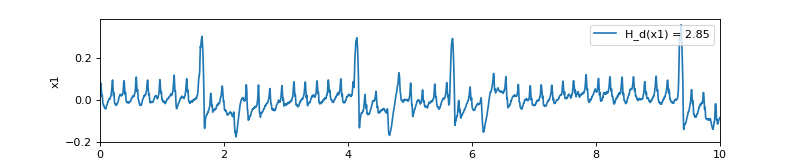
Examples

import numpy as np
import matplotlib.pyplot as plt
import spkit as sp
np.random.seed(1)
x1, fs = sp.data.optical_sample(sample=1)
t = np.arange(len(x1))/fs
H_de1, prob1  = sp.dispersion_entropy_multiscale_refined(x1,classes=10,scales=[1,2,3,4,5,6,7,8])
print('DE of x1 = ',H_de1)
plt.figure(figsize=(10,2))
plt.plot(t,x1, label=f'H_d(x1) = {H_de1:,.2f}')
plt.xlim([t[0],t[-1]])
plt.ylabel('x1')
plt.xlabel('time (s)')
plt.legend(loc='upper right')
plt.show()