spkit.stft_analysis

spkit.stft_analysis(x, winlen, window='blackmanharris', nfft=None, overlap=None, plot=False, fs=1, interpolation=None, figsize=(10, 5))

Short-Time Fourier Transform Analysis Model

Analysis of a signal using the Short-Time Fourier Transform

Parameters:

x: 1d-array

• signal - shape (n,)

winlenint,

• window length for analysis (good choice is a odd number)

• window size is chosen based on the frequency resolution required

• winlen >= Bs*fs/del_f

• where Bs=4 for hamming window, Bs=6 for blackman harris

• def_f is different between two frequecies (to be resolve)

• higher the window length better the frequency resolution, but poor time resolution

overlap: int, default = None

• overlap of windows

• if None then winlen//2 is used (50% overlap)

• shorter overlap can improve time resoltion - upto an extend

window: str, default = blackmanharris

• analysis window

• if None, rectangular window is used

nfft: int,

• FFT size, should be >=winlen and power of 2

• if None - nfft = 2**np.ceil(np.log2(len(n)))

plot: bool, (default: False)

• False, for no plot

• True for plot

fsint, deafult=None

• sampling frequency, only used for plots

• if not provided, fs=1 is used

• it does not affect any computations

interpolation: str, default=None, {‘bilinear’, ‘sinc’, ..}

• interpolation applied to plot

• it does not affect any computations

figsize: figure-size

Returns:

mXt2d-array,

• magnitude spectra of shape (number of frames, int((nfft/2)+1))

pXt2d-array,

• phase spectra of same shape as mXt

See also

stft_synthesis

Inverse Short-Time Fourier Transform - iSTFT

dft_analysis

Discreet Fourier Transform - DFT

dft_synthesis

Inverse Discreet Fourier Transform - iDFT

frft

Fractional Frourier Transform - FRFT

ifrft

Inverse Fractional Frourier Transform - iFRFT

sineModel_analysis

Sinasodal Model Decomposition

sineModel_synthesis

Sinasodal Model Synthesis

Examples

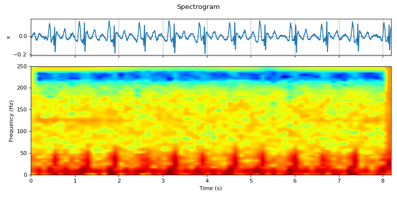
#sp.stft_analysis
import numpy as np
import matplotlib.pyplot as plt
import spkit as sp
x,fs,lead_names = sp.data.ecg_sample_12leads(sample=2)
x = x[:int(fs*10),5]
x = sp.filterDC_sGolay(x, window_length=fs//3+1)
t = np.arange(len(x))/fs
mXt, pXt = sp.stft_analysis(x,winlen=127)
fig, (ax1, ax2) = plt.subplots(2, 1, gridspec_kw={'height_ratios': [1, 3]},figsize=(10,5))
ax1.plot(t,x)
ax1.set_xlim([t[0],t[-1]])
ax1.set_ylabel('x')
ax1.grid()
ax1.set_xticklabels('')
ax2.imshow(mXt.T,aspect='auto',origin='lower',cmap='jet',extent=[t[0],t[-1],0,fs/2],interpolation='bilinear')
ax2.set_ylabel('Frequency (Hz)')
ax2.set_xlabel('Time (s)')
fig.suptitle('Spectrogram')
plt.tight_layout()
plt.show()

#####################
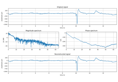
#sp.stft_analysis
import numpy as np
import matplotlib.pyplot as plt
import spkit as sp
x,fs,lead_names = sp.data.ecg_sample_12leads(sample=2)
x = x[:int(fs*10),5]
x = sp.filterDC_sGolay(x, window_length=fs//3+1)
t = np.arange(len(x))/fs
mXt, pXt = sp.stft_analysis(x,winlen=127,plot=True, fs=fs)

Examples using spkit.stft_analysis

Analysis and Synthesis Models

Analysis and Synthesis Models

Sinusoidal Model : Synthesis : Audio

Sinusoidal Model : Synthesis : Audio

Sinusoidal Model: Analysis and Synthesis

Sinusoidal Model: Analysis and Synthesis