spkit.dft_synthesis

spkit.dft_synthesis(mX, pX, M=None, scaling_dB=True, window=None)

Discrete Fourier Transform: Synthesis (iDFT)

Synthesis of a signal using the Discrete Fourier Transform from positive spectra

Parameters:

mX: 1d-array

• magnitude spectrum - (of shape=int((N/2)+1)) for N-point FFT (output of dft_synthesis)

pX: same size as mX

• phase spectrum (output of dft_synthesis)

Mint, deafult=None

• length of signal: x, if None, then M = N = 2*(len(mX)-1)

window: default=None

• rescaling signal, undoing the scaling

• if provided, synthesized signal is rescalled with corresponding window function

• if None, then reconstructed signal will have different scale than original signal,

• reconstructed signal will still have windowing effect, if window was used other than ‘boxcar’ - rectangual

scaling_dB, bool, deafult=True,

• if false, then linear scale of spectrum is assumed, else in dB

Returns:

y: output signal of shape (M,)

See also

dft_analysis

Discreet Fourier Transform - DFT

stft_analysis

Short-Time Fourier Transform - STFT

stft_synthesis

Inverse Short-Time Fourier Transform - iSTFT

frft

Fractional Frourier Transform - FRFT

ifrft

Inverse Fractional Frourier Transform - iFRFT

sineModel_analysis

Sinasodal Model Decomposition

sineModel_synthesis

Sinasodal Model Synthesis

Notes

#TODO

References

• wikipedia - https://en.wikipedia.org/wiki/Discrete_Fourier_transform

Examples

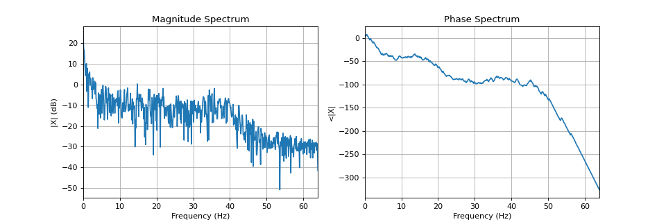
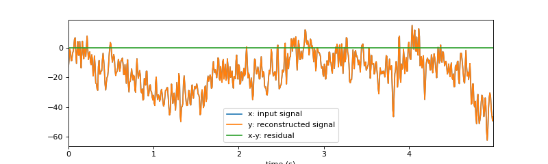
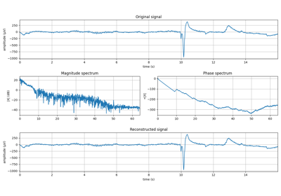
#sp.dft_synthesis
import numpy as np
import matplotlib.pyplot as plt
import spkit as sp
x,fs = sp.data.eeg_sample_1ch(ch=1)
x = x[:int(fs*5)]
t = np.arange(len(x))/fs
mX, pX, N = sp.dft_analysis(x,plot=True,fs=fs,window='boxcar')
y = sp.dft_synthesis(mX,pX,M=len(x),window='boxcar')
plt.figure(figsize=(10,3))
plt.plot(t,x,label='x: input signal')
plt.plot(t,y,label='y: reconstructed signal')
plt.plot(t,x-y,label='x-y: residual')
plt.xlim([t[0],t[-1]])
plt.xlabel('time (s)')
plt.legend()
plt.show()

Examples using spkit.dft_synthesis

Analysis and Synthesis Models

Analysis and Synthesis Models