spkit.ifrft
- spkit.ifrft(x, alpha=0.1, method=1, verbose=0)
Inverse Fractional Fourier Transform
Inverse Fractional Fourier Transform
- Parameters:
- x: complex-signal
- alpha: scalar, 0<a<4
- method=1, other methods to be implemented
- Returns:
- y: complex signal
- reconstruction using IFRFT
- imaginary part is mostly zero
See also
Notes
# Recostruction of the signal is has some artifact to be removed.
References
wikipedia
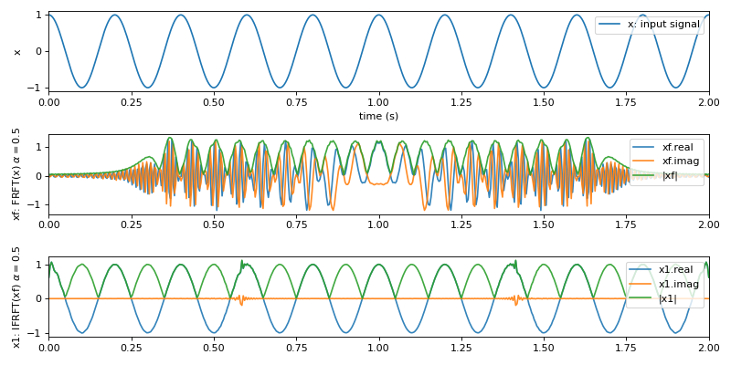
Examples
#sp.ifrft
import numpy as np
import matplotlib.pyplot as plt
import spkit as sp
t = np.linspace(0,2,500)
x = np.cos(2*np.pi*5*t)
xf = sp.frft(x,alpha=0.5)
x1 = sp.ifrft(xf,alpha=0.5)
plt.figure(figsize=(10,5))
plt.subplot(311)
plt.plot(t,x,label='x: input signal')
plt.xlim([t[0],t[-1]])
plt.xlabel('time (s)')
plt.ylabel('x')
plt.legend(loc='upper right')
plt.subplot(312)
plt.plot(t,xf.real,label='xf.real',alpha=0.9)
plt.plot(t,xf.imag,label='xf.imag',alpha=0.9)
plt.plot(t,np.abs(xf),label='|xf|',alpha=0.9)
plt.xlim([t[0],t[-1]])
plt.ylabel(r'xf: FRFT(x) $\alpha=0.5$')
plt.legend(loc='upper right')
plt.subplot(313)
plt.plot(t,x1.real,label='x1.real',alpha=0.9)
plt.plot(t,x1.imag,label='x1.imag',alpha=0.9)
plt.plot(t,np.abs(x1),label='|x1|',alpha=0.9)
plt.xlim([t[0],t[-1]])
plt.ylabel(r'x1: IFRFT(xf) $\alpha=0.5$')
plt.legend(loc='upper right')
plt.tight_layout()
plt.show()