spkit.dominent_freq_win
- spkit.dominent_freq_win(X, fs, win_len=100, overlap=None, method='welch', refine_peak=False, nfft=None, nperseg=None, exclude_lower_fr=None, window='hann', use_joblib=False, verbose=1, **kwargs)
Dominent Frequency Analysis Window-wise
This function computes dominent frequency in moving window, to analyse the dynamics dominent frequency.
- Parameters:
- X: 1d-array 2d-array
input signal, for 2d, channel axis is 1, e.g., (n,ch)
single channel or multichannel signal
- fs: int,
sampling frequency
- win_len: int, deault=100
length of window
- overlap: int, or None
if None, overlap=win_len//2
- method: str, {‘welch’,’fft’,None}, deafult=’welch’
method to compute spectrum
welch method is prefered, (see example), uses scipy.signal.welch
if None or other than ‘welch’ and ‘fft’, periodogram is used to compute spectum ( scipy.signal.peridogram)
if ‘fft’ or ‘FFT’,
dft_analysisis used.
- window: str, default=’hann’
windowing function
- exclude_lower_fr: None or scalar
if not None, any peak before exclude_lower_fr is excluded
useful to avoid dc component or any known low-frequency component
example: exclude_lower_fr=2, will exclude all the peaks before 2Hz
- refine_peak: bool, default=False
if True, peak is refined using parobolic interpolation
- return_spectrum: bool, default=False
if True, Magnitude spectrum and frequency values are returned along with dominent frequency
useful to analyse
- (nfft,nperseg): parameters for ‘welch’ and ‘periodogram’ method
- **kwargs:
- any aaditional keywords to pass to scipy.signal.welch or scipy.signal.periodogram
method.
- verbose: int
verbosity level, 0: silence
- Returns:
- DF_win: array
Dominent Frequencies of each window, size of (nw, ch),
See also
clean_phase,phase_map,dominent_freq,phase_map_reconstruction,amplitude_equalizer
Notes
For details, chekc
dominent_freqReferences
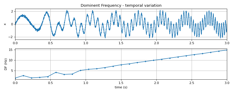
Examples
#sp.dominent_freq_win
import numpy as np
import matplotlib.pyplot as plt
import spkit as sp
fs=500
t = np.linspace(0,3,7*fs)
f=3
x = np.sin(2*np.pi*f*t) + np.sin(2*np.pi*2*f*t**2)
x = sp.add_noise(x,snr_db=20)
df_win = sp.dominent_freq_win(x,fs,win_len=fs//2,refine_peak=True,verbose=0)
tx = t[-1]*np.arange(len(df_win))/(len(df_win)-1)
plt.figure(figsize=(10,4))
plt.subplot(211)
plt.plot(t,x)
plt.ylabel('x')
plt.xlim([t[0],t[-1]])
plt.grid()
plt.title('Dominent Frequency - temporal variation')
plt.subplot(212)
plt.plot(tx,df_win,marker='.')
plt.xlim([t[0],t[-1]])
plt.ylabel('DF (Hz)')
plt.xlabel('time (s)')
plt.grid()
plt.subplots_adjust(hspace=0)
plt.tight_layout()
plt.show()