spkit.phase_map
- spkit.phase_map(X, add_sig=False)
Phase Mapping of multi channel signals X
Phase computation
\[\theta = tan^{-1}(A_y/A_x)\]# Analytical Signal using Hilbert Transform
\[A_x + j*A_y = HT(x)\]if add_sig True
- Parameters:
- X(n,ch) shape= (samples, n_channels)
- add_sig: bool, False,
if True: \(A_x + j*A_y = x + j*HT(x)\)
else: \(A_x + j*A_y = HT(x)\)
- Returns:
- PM(n,ch) shape= (samples, n_channels)
See also
clean_phase,dominent_freq,phase_map_reconstruction,dominent_freq_win,amplitude_equalizer
Notes
#TODO
References
wikipedia - https://en.wikipedia.org/wiki/Analytic_signal
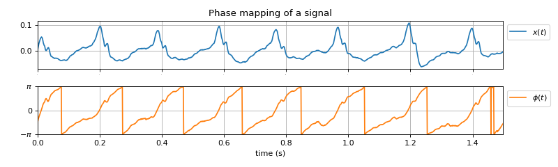
Examples
>>> #sp.phase_map
>>> import numpy as np
>>> import matplotlib.pyplot as plt
>>> import spkit as sp
>>> x,fs = sp.data.optical_sample(sample=1)
>>> x = x[:int(1.5*fs)]
>>> x = sp.filterDC_sGolay(x,window_length=fs//2+1)
>>> t = np.arange(len(x))/fs
>>> xp = sp.phase_map(x,add_sig=False)
>>> plt.figure(figsize=(10,3))
>>> plt.subplot(211)
>>> plt.plot(t,x,label=f'$x(t)$')
>>> plt.grid()
>>> plt.legend(bbox_to_anchor=(1,1))
>>> plt.xlim([t[0],t[-1]])
>>> plt.xticks(fontsize=0)
>>> plt.title('Phase mapping of a signal')
>>> plt.subplot(212)
>>> plt.plot(t,xp,color='C1',label=r'$\phi (t)$')
>>> plt.xlim([t[0],t[-1]])
>>> plt.ylim([-np.pi,np.pi])
>>> plt.yticks([-np.pi,0,np.pi],[r'$-\pi$','0',r'$\pi$'])
>>> plt.ylabel('')
>>> plt.xlabel('time (s)')
>>> plt.grid()
>>> plt.legend(bbox_to_anchor=(1,1))
>>> plt.subplots_adjust(hspace=0)
>>> plt.tight_layout()
>>> plt.show()