spkit.dominent_freq
- spkit.dominent_freq(X, fs, method='welch', window='hann', exclude_lower_fr=None, refine_peak=False, nfft=None, nperseg=None, return_spectrum=False, **kwargs)
Dominent Frequency Analysis
Dominent Frequency Analysis is one of the approach used to discern the different physiology from a biomedical signals [1].
This function compute dominent frequency as the maximum peak in the spectrum. The location of the peak is returned in Hz
The value of dominent frquency depends on the computing method for spectrum. Using Welch method is prefered as it computes Other posible approaches are ‘FFT’ and ‘Periodogram’
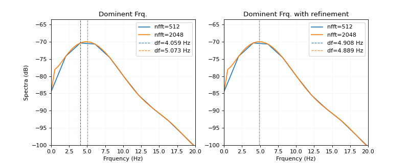
Computed peak can further be refined using parobolic interpolation.
- Parameters:
- X: 1d-array 2d-array
input signal, for 2d, channel axis is 1, e.g., (n,ch)
single channel or multichannel signal
- fs: int,
sampling frequency
- method: str, {‘welch’,’fft’,None}, deafult=’welch’
method to compute spectrum
welch method is prefered, (see example), uses scipy.signal.welch
if None or other than ‘welch’ and ‘fft’, periodogram is used to compute spectum ( scipy.signal.peridogram)
if ‘fft’ or ‘FFT’,
dft_analysisis used.
- window: str, default=’hann’
windowing function
- exclude_lower_fr: None or scalar
if not None, any peak before exclude_lower_fr is excluded
useful to avoid dc component or any known low-frequency component
example: exclude_lower_fr=2, will exclude all the peaks before 2Hz
- refine_peak: bool, default=False
if True, peak is refined using parobolic interpolation
- return_spectrum: bool, default=False
if True, Magnitude spectrum and frequency values are returned along with dominent frequency
useful to analyse
- (nfft,nperseg): parameters for ‘welch’ and ‘periodogram’ method
- **kwargs:
- any aaditional keywords to pass to scipy.signal.welch or scipy.signal.periodogram
method.
- Returns:
- DF: scalar or 1d-array
scalar of X is 1d
array of scalers of length ch, if X is 2d
- (mX, Frq)Spectrum, if return_spectrum is True
See also
clean_phase,phase_map,phase_map_reconstruction,dominent_freq_win,amplitude_equalizer
Notes
Refining peak achive better localization of dominence in spectrum. See Example.
References
Examples
#sp.dominent_freq
import numpy as np
import matplotlib.pyplot as plt
import spkit as sp
import scipy
x,fs = sp.data.optical_sample(sample=1)
x = x[:int(5*fs)]
x = sp.filterDC_sGolay(x,window_length=fs//2+1)
t = np.arange(len(x))/fs
dfq = sp.dominent_freq(x,fs,method='welch',refine_peak=True)
print('Dominent Frequency: ',dfq,'Hz')
dfq1, (mX1, frq1) = sp.dominent_freq(x,fs,method='welch',nfft=512,return_spectrum=True)
dfq2, (mX2, frq2) = sp.dominent_freq(x,fs,method='welch',nfft=2048,return_spectrum=True)
dfq3, (mX3, frq3) = sp.dominent_freq(x,fs,method='welch',nfft=512,return_spectrum=True,refine_peak=True)
dfq4, (mX4, frq4) = sp.dominent_freq(x,fs,method='welch',nfft=2048,return_spectrum=True,refine_peak=True)

plt.figure(figsize=(10,4))
plt.subplot(121)
plt.plot(frq1, 20*np.log10(mX1), label='nfft=512')
plt.plot(frq2, 20*np.log10(mX2), label='nfft=2048')
plt.axvline(dfq1,color='C0',ls='--',lw=1,label=f'df={dfq1:.3f} Hz')
plt.axvline(dfq2,color='C1',ls='--',lw=1,label=f'df={dfq2:.3f} Hz')
plt.xlim([0,20])
plt.ylim([-100, None])
plt.grid(alpha=0.1)
plt.ylabel('Spectra (dB)')
plt.xlabel('Frquency (Hz)')
plt.title('Dominent Frq.')
plt.legend()
plt.subplot(122)
plt.plot(frq3, 20*np.log10(mX3), label='nfft=512')
plt.plot(frq4, 20*np.log10(mX4), label='nfft=2048')
plt.axvline(dfq3,color='C0',ls='--',lw=1,label=f'df={dfq3:.3f} Hz')
plt.axvline(dfq4,color='C1',ls='--',lw=1,label=f'df={dfq4:.3f} Hz')
plt.xlim([0,20])
plt.ylim([-100, None])
plt.grid(alpha=0.1)
plt.xlabel('Frquency (Hz)')
plt.title('Dominent Frq. with refinement')
plt.legend()
plt.show()