Note

Go to the end to download the full example code or to run this example in your browser via JupyterLite or Binder

Decision Trees with shrinking capability - Classification example¶

Decision Trees with shrinking capability from SpKit (Classification example)

In this notebook, we show the capability of decision tree from *spkit* to analysie the training and testing performace at each depth of a trained tree. After which, a trained tree can be shrink to any smaller depth, *without retraining it*. So, by using Decision Tree from *spkit*, you could choose a very high number for a max_depth (or just choose -1, for infinity) and analysis the parformance (accuracy, mse, loss) of training and testing (practically, a validation set) sets at each depth level. Once you decide which is the right depth, you could shrink your trained tree to that layer, without explicit training it again to with new depth parameter.

spkit version : 0.0.9.7
(442, 10) (442,)
(309, 10) (133, 10) (309,) (133,)
Depth of trained Tree  12
Accuracy
- Training :  1.0
- Testing  :  0.7218045112781954
Logloss
- Training :  -1.0000000826903709e-10
- Testing  :  6.405687852618023
{'measure': 'acc', 1: {'train': 0.7378640776699029, 'test': 0.7142857142857143}, 2: {'train': 0.7378640776699029, 'test': 0.7142857142857143}, 3: {'train': 0.7831715210355987, 'test': 0.7218045112781954}, 4: {'train': 0.8252427184466019, 'test': 0.6842105263157895}, 5: {'train': 0.8543689320388349, 'test': 0.7142857142857143}, 6: {'train': 0.8867313915857605, 'test': 0.706766917293233}, 7: {'train': 0.9158576051779935, 'test': 0.7518796992481203}, 8: {'train': 0.9385113268608414, 'test': 0.7518796992481203}, 9: {'train': 0.9676375404530745, 'test': 0.7218045112781954}, 10: {'train': 0.9838187702265372, 'test': 0.7218045112781954}, 11: {'train': 0.9935275080906149, 'test': 0.7218045112781954}, 12: {'train': 1.0, 'test': 0.7218045112781954}}
Depth of trained Tree  7
Accuracy
- Training :  0.9158576051779935
- Testing  :  0.7518796992481203
Logloss
- Training :  0.19382486739414417
- Testing  :  3.3542011731632746

import numpy as np
import matplotlib.pyplot as plt
from sklearn.model_selection import train_test_split
import spkit
print('spkit version :', spkit.__version__)

# just to ensure the reproducible results
np.random.seed(100)

# Classification  - Diabetes Dataset -  binary class

from spkit.ml import ClassificationTree

# Diabetes Dataset
from sklearn.datasets import load_diabetes
data = load_diabetes()
X = data.data
y = 1*(data.target>np.mean(data.target))

feature_names = data.feature_names
print(X.shape, y.shape)
Xt,Xs,yt,ys = train_test_split(X,y,test_size =0.3)
print(Xt.shape, Xs.shape,yt.shape, ys.shape)


# Train with max_depth =15, Accuracy, Logloss

model = ClassificationTree(max_depth=15)
model.fit(Xt,yt,feature_names=feature_names)
ytp = model.predict(Xt)
ysp = model.predict(Xs)

ytpr = model.predict_proba(Xt)[:,1]
yspr = model.predict_proba(Xs)[:,1]

print('Depth of trained Tree ', model.getTreeDepth())
print('Accuracy')
print('- Training : ',np.mean(ytp==yt))
print('- Testing  : ',np.mean(ysp==ys))
print('Logloss')
Trloss = -np.mean(yt*np.log(ytpr+1e-10)+(1-yt)*np.log(1-ytpr+1e-10))
Tsloss = -np.mean(ys*np.log(yspr+1e-10)+(1-ys)*np.log(1-yspr+1e-10))
print('- Training : ',Trloss)
print('- Testing  : ',Tsloss)


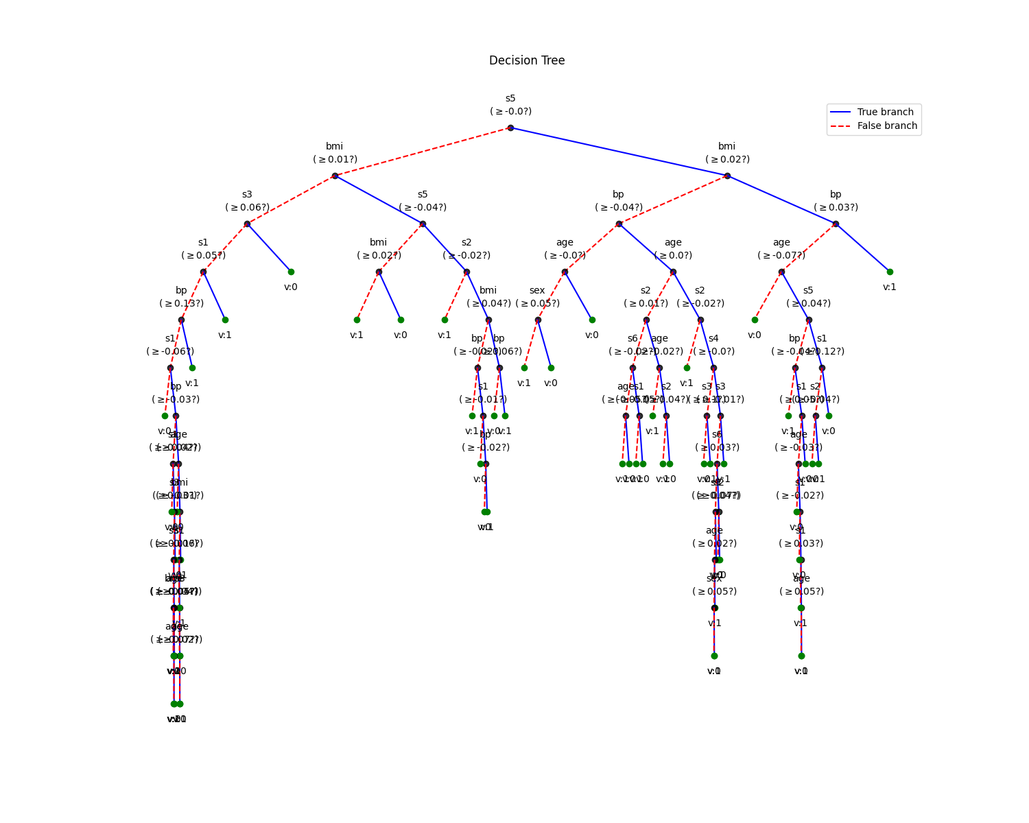
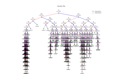
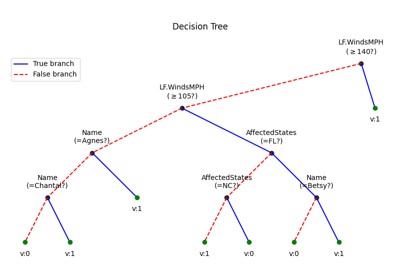
# Plot Trained Tree

plt.figure(figsize=(15,12))
model.plotTree()


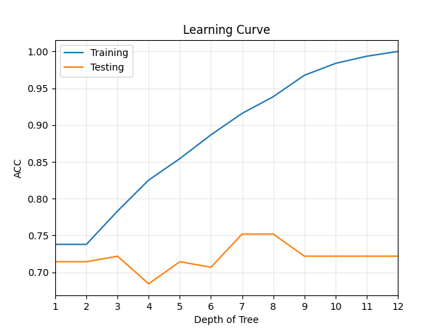
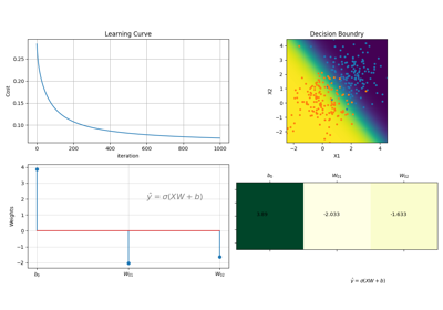
# Analysing the Learning Curve with test data (validation set)

Lcurve = model.getLcurve(Xt=Xt,yt=yt,Xs=Xs,ys=ys,measure='acc')
print(Lcurve)

model.plotLcurve()
plt.xlim([1,model.getTreeDepth()])
plt.xticks(np.arange(1,model.getTreeDepth()+1))
plt.show()


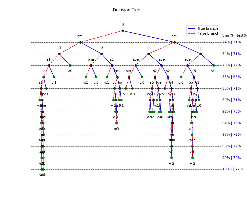
# Learning curve with tree

plt.figure(figsize=(10,8))
model.plotTree(show=False,Measures=True,showNodevalues=True,showThreshold=False)


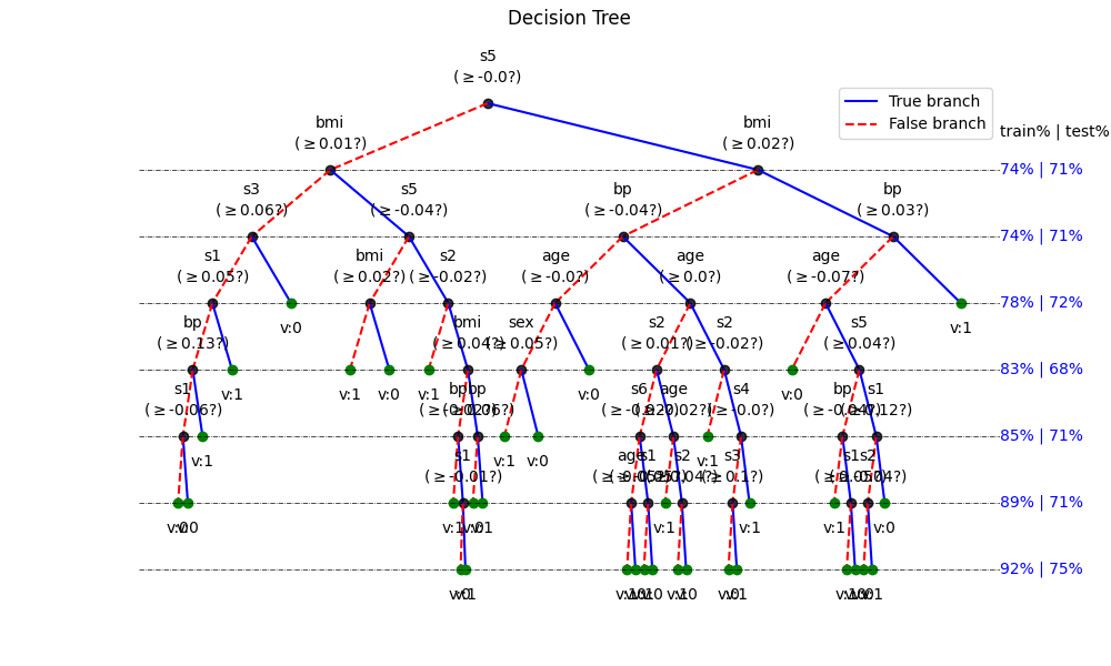
# Shrinking the trained tree to depth=7

model.updateTree(shrink=True,max_depth=7)


ytp = model.predict(Xt)
ysp = model.predict(Xs)

ytpr = model.predict_proba(Xt)[:,1]
yspr = model.predict_proba(Xs)[:,1]

print('Depth of trained Tree ', model.getTreeDepth())
print('Accuracy')
print('- Training : ',np.mean(ytp==yt))
print('- Testing  : ',np.mean(ysp==ys))
print('Logloss')
Trloss = -np.mean(yt*np.log(ytpr+1e-10)+(1-yt)*np.log(1-ytpr+1e-10))
Tsloss = -np.mean(ys*np.log(yspr+1e-10)+(1-ys)*np.log(1-yspr+1e-10))
print('- Training : ',Trloss)
print('- Testing  : ',Tsloss)


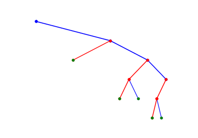
# # Plotting final tree

plt.figure(figsize=(10,6))
model.plotTree(show=False,Measures=True,showNodevalues=True,showThreshold=True)