Note

Go to the end to download the full example code or to run this example in your browser via JupyterLite or Binder

Decision Trees without converting Catogorical Features¶

Decision Trees without converting Catogorical Features using SpKit

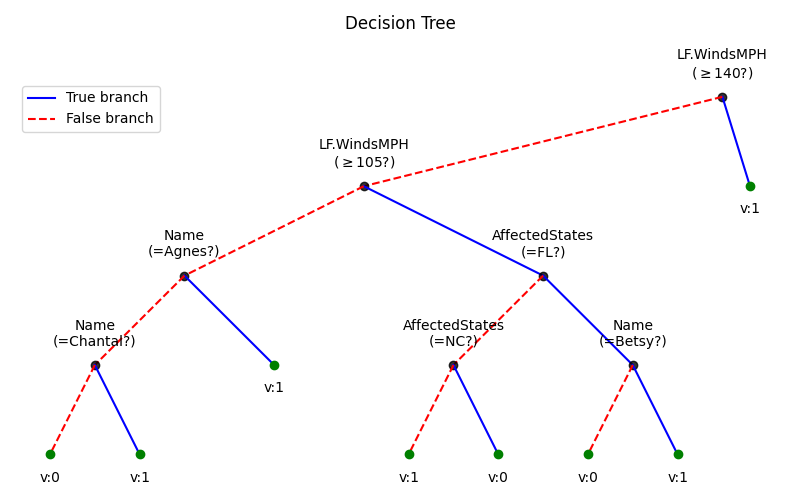
Most of ML libraries force us to convert the catogorycal features into one-hot vector or any numerical value. However, it should not be the case, Not atleast with Decision Trees, due a simple reason, of how decision tree works. In spkit library, Decision tree can handle mixed type input features, ‘Catogorical’ and ‘Numerical’. In this notebook, I would use a dataset hurricNamed from vincentarelbundock github repository, and use only a few features, mixed of catogorical and numerical features. Converting number of deaths to binary with threshold of 10, we handle this as Classification Problem. However, it is not shown that coverting features into one-hot vector or any label encoder affects the performance of model, but, it is useful, when you need to visulize the decision process. Very important when you need to extract and simplify the decision rule.

spkit version : 0.0.9.7
Shapes (94, 4) (94,)

import numpy as np
import pandas as pd
import matplotlib.pyplot as plt
import spkit
print('spkit version :', spkit.__version__)


# just to ensure the reproducible results
np.random.seed(100)

# ## Classification  - binary class - hurricNamed Dataset

from spkit.ml import ClassificationTree


D = pd.read_csv('https://vincentarelbundock.github.io/Rdatasets/csv/DAAG/hurricNamed.csv')
feature_names = ['Name', 'AffectedStates','LF.WindsMPH','mf']#,'BaseDamage' 'Year','Year','LF.WindsMPH', 'LF.PressureMB','LF.times',


X = np.array(D[feature_names])
X[:,1] = [st.split(',')[0] for st in X[:,1]] #Choosing only first name of state from AffectedStates feature
y = np.array(D[['deaths']])[:,0]

# Converting target into binary with threshold of 10 deaths
y[y<10] =0
y[y>=10]=1


print('Shapes',X.shape,y.shape)


# ## Training,

# Not doing training and testing, as objective is to show that it works

model = ClassificationTree(max_depth=4)
model.fit(X,y,feature_names=feature_names)
yp = model.predict(X)


plt.figure(figsize=(8,5))
model.plotTree()
plt.tight_layout()
plt.show()


# Here, it can be seen that first feature 'LF.WindsMPH' is a numerical, thus the threshold is greater then equal to, however for catogorical features like 'Name' and 'AffectedStates'threshold is equal to only.