
1.1. Entropy
Entropy (Entropie - greek) is the fundamental concept in infromation theory. The term is associated with state of disorder, uncertainity or randomness. The term was first introduced in the field of thermo dynamics (during 1803-1877) and later in 1948, Claude Shannon introduced it - information entropy as a measure of ‘information’, ‘uncertianity’ or ‘surprise’ [1]_.
Consider a discreet random variable \(X\), drawn from a source \(S\) with probability distribuation as \(\mathcal{X} \rightarrow [0,1]\), the entropy of random variable \(X\) is:
1.1.1. Entropy with discreet source
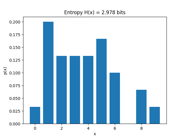
entropy computes entropy \(H(x)\) using probability distribution for
\(\sum p(x) log \left( p(x) \right)\).
For a discreet source, computing probability distribution is quite straighforward. entropy uses
numpy’s unique to compute frequency np.unique and uses it to compute probability distribuation p(x)
entropy is a generalised for function, to compute entropy of a discreet variable, is_discrete argument has to be set to True.
>>> import numpy as np
>>> import spkit as sp
>>> x = np.array([4,4,4,2,2,2,1])
>>> Hx = sp.entropy(x,is_discrete=True)
1.4488156358175899
In this example, the probability of random variable \(x\) is \(p(1) = 1/7\), \(p(2) = 3/7\), \(p(4) = 3/7\).
Using \(\sum p(x)log \left( p(x) \right)\). it computes to 1.4488156357251847
For numerical stability, entropy adds 1e-10 to p, which leads a very small difference.
1.1.1.1. Change of base
While it is common to use the base 2 for log, which compute entropy is bits.
It is possible to change the base of log in the computatation by changing the default value of base=2.
>>> Hx = sp.entropy(x,is_discrete=True, base='e')
>>> Hx = sp.entropy(x,is_discrete=True, base=10)
with base e unit of entropy is ‘nat’ (natural unit) and with base 10 unit is ‘dits’ (or ‘bans’ or ‘hartleys’).
Check here for more details : Base of log in Entropy [2]_.
1.1.2. Rényi entropy of order \(\alpha\)
Rényi entropy is generalised form of entropy which includes various notion of entropy functions [3]_. Shannon entropy, Hartley entropy, and collision entropy are the special case of it. Rényi entropy of order \(\alpha\) is defined as:
for \(0 < \alpha < \infty\) and \(\alpha \ne 1\)
spkit entropy function is equiped to change compute the Rényi entropy by setting value of \(\alpha\).
For \(\alpha = 0\): Maximum Entropy (Hartley entropy)
For \(\alpha = \infty\): Minmum Entropy
For \(\alpha = 1\): Shannon Entropy (default)
For \(\alpha = 2\): Rényi entropy of order \(\alpha\) (collision entropy)
Here are the examples
>>> import numpy as np
>>> import spkit as sp
>>> x = np.array([4,4,4,2,2,2,1])
>>> Hx = sp.entropy(x,is_discrete=True, alpha=0)
>>> print('Entropy with alpha = 0', Hx)
1.5849625007211563
>>> Hx = sp.entropy(x,is_discrete=True, alpha=0.5)
>>> print('Entropy with alpha = 0.5', Hx)
1.5093848128656548
>>> Hx = sp.entropy(x,is_discrete=True, alpha=1)
>>> print('Entropy with alpha = 1', Hx)
1.4488156358175899
>>> Hx = sp.entropy(x,is_discrete=True, alpha=2)
>>> print('Entropy with alpha = 2', Hx)
1.366782329927496
>>> Hx = sp.entropy(x,is_discrete=True, alpha=10)
>>> print('Entropy with alpha = 10', Hx)
1.2471013326629172
>>> Hx = sp.entropy(x,is_discrete=True, alpha='inf')
>>> print("Entropy with alpha = 'inf'", Hx)
11.2223924209998192
References
Click for more details
1.1.3. Entropy for real-valued source
1.1.4. Shannon Entropy \(H(X)\)
>>> import numpy as np
>>> import spkit as sp
>>> np.random.seed(1)
>>> x = np.random.rand(10000)
>>> y = np.random.randn(10000)
>>> #Shannan entropy
>>> H_x = sp.entropy(x,alpha=1)
>>> H_y = sp.entropy(y,alpha=1)
>>> print('Shannan entropy')
>>> print('Entropy of x: H(x) = ',H_x)
>>> print('Entropy of y: H(y) = ',H_y)
>>> print('')
>>> Hn_x = sp.entropy(x,alpha=1, normalize=True)
>>> Hn_y = sp.entropy(y,alpha=1, normalize=True)
>>> print('Normalised Shannan entropy')
>>> print('Entropy of x: H(x) = ',Hn_x)
>>> print('Entropy of y: H(y) = ',Hn_y)
>>> np.random.seed(None)
    Shannan entropy
    Entropy of x: H(x) =  4.458019387223165
    Entropy of y: H(y) =  5.043357283463282
    ----
    Normalised Shannan entropy
    Entropy of x: H(x) =  0.9996833158270148
    Entropy of y: H(y) =  0.8503760993630085
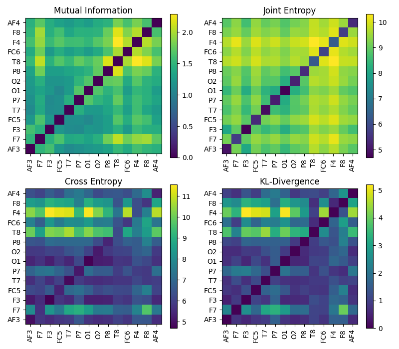
1.1.5. Mutual Information \(I(X;Y)\)
\[I(X;Y) = H(X) + H(Y) - H(X,Y)\]\[I(X;Y) = H(X) - H(X|Y)\]\[0 <= I(X;Y) <= min\{ H(x), H(y)\}\]

One example of computing mutual information is as follow;
>>> import numpy as np
>>> import matplotlib.pyplot as plt
>>> import spkit as sp
>>> np.random.seed(1)
>>> x = np.random.randn(1000)
>>> y1 = 0.1*x + 0.9*np.random.randn(1000)
>>> y2 = 0.9*x + 0.1*np.random.randn(1000)
>>> I_xy1 = sp.mutual_info(x,y1)
>>> I_xy2 = sp.mutual_info(x,y2)
>>> sp.mutual_info(x,y1)
>>> print(r'I(x,y1) = ',I_xy1, '\t| y1 /= e x')
>>> print(r'I(x,y2) = ',I_xy2, '\t| y2 ~ x')
>>> np.random.seed(None)
1.1.6. Joint-Entropy \(H(X;Y)\)

An example to compute Joint Entropy is as follow;
>>> import numpy as np
>>> import matplotlib.pyplot as plt
>>> import spkit as sp
>>> X, fs, ch_names = sp.data.eeg_sample_14ch()
>>> x,y1 = X[:,0],X[:,5]
>>> H_xy1= sp.entropy_joint(x,y1)
>>> print('Joint Entropy')
>>> print(f'- H(x,y1) = {H_xy1}')
1.1.7. Conditional Entropy \(H(X|Y)\)

An example to compute Joint Entropy is as follow;
>>> import numpy as np
>>> import spkit as sp
>>> X, fs, ch_names = sp.data.eeg_sample_14ch()
>>> X = X - X.mean(1)[:, None]
>>> x,y1 = X[:,0],X[:,5]
>>> y2 = sp.add_noise(y1,snr_db=0)
>>> H_x = sp.entropy(x)
>>> H_x1y1= sp.entropy_cond(x,y1)
>>> H_x1y2= sp.entropy_cond(x,y2)
>>> print('Conditional Entropy')
>>> print(f'- H(x|y1) = {H_x1y1}')
>>> print(f'- H(x|y2) = {H_x1y2}')
>>> print(f'- H(x) = {H_x}')
1.1.8. Cross Entropy \(H_{xy}(X,Y)\)
Cross Entropy
An example is as follow:
>>> import numpy as np
>>> import spkit as sp
>>> np.random.seed(1)
>>> X, fs, ch_names = sp.data.eeg_sample_14ch()
>>> X = X - X.mean(1)[:, None]
>>> x,y1 = X[:,0],X[:,5]
>>> y2 = sp.add_noise(y1,snr_db=0)
>>> H_x = sp.entropy(x)
>>> H_xy1= sp.entropy_cross(x,y1)
>>> H_xy2= sp.entropy_cross(x,y2)
>>> print('Cross Entropy')
>>> print(f'- H_(x,y1) = {H_xy1}')
>>> print(f'- H_(x,y2) = {H_xy2}')
>>> print(f'- H(x) = {H_x}')
>>> np.random.seed(None)
1.1.9. Cross Entropy: KL-Divergence \(H_{kl}(X,Y)\)
Cross Entropy - Kullback–Leibler divergence
An example is as follow:
>>> import numpy as np
>>> import spkit as sp
>>> np.random.seed(1)
>>> X, fs, ch_names = sp.data.eeg_sample_14ch()
>>> X = X - X.mean(1)[:, None]
>>> x,y1 = X[:,0],X[:,5]
>>> y2 = sp.add_noise(y1,snr_db=0)
>>> H_x = sp.entropy(x)
>>> H_xy1= sp.entropy_kld(x,y1)
>>> H_xy2= sp.entropy_kld(x,y2)
>>> print('Cross Entropy - KL')
>>> print(f'- H_kl(x,y1) = {H_xy1}')
>>> print(f'- H_kl(x,y2) = {H_xy2}')
>>> print(f'- H(x) = {H_x}')
>>> np.random.seed(None)
1.1.10. Approximate Entropy \(H_{ae}(X)\)
Approximate Entropy \(ApproxEn(X)\) or \(H_{ae}(X)\)
Approximate entropy is more suited for temporal source, (non-IID), such as physiological signals, or signals in general. Approximate entropy like Sample Entropy (
entropy_sample) measures the complexity of a signal by extracting the pattern of m-symbols.mis also called as embedding dimension.ris the tolarance here, which determines the two patterns to be same if their maximum absolute difference is thanr.
Aproximate Entropy is Embeding based entropy function. Rather than considering a signal sample, it consider the m-continues samples (a m-deminesional temporal pattern) as a symbol generated from a process. This set of “m-continues samples” is considered as “Embeding” and then estimating distribuation of computed symbols (embeddings). In case of a real valued signal, two embeddings will rarely be an exact match, so, the factor r is defined as if two embeddings are less than r distance away to each other, they are considered as same. This is a way to quantization of embedding and limiting the Embedding Space.
For Aproximate Entropy the value of r depends the application and the order (range) of signal. One has to keep in mind that r is the distance be between two Embeddings (m-deminesional temporal pattern). A typical value of r can be estimated on based of SD of x ~ 0.2*std(x).
>>> import numpy as np
>>> import spkit as sp
>>> t = np.linspace(0,2,200)
>>> x1 = np.sin(2*np.pi*1*t) + 0.1*np.random.randn(len(t))  # less noisy
>>> x2 = np.sin(2*np.pi*1*t) + 0.5*np.random.randn(len(t))  # very noisy
>>> #Approximate Entropy
>>> H_x1 = sp.entropy_approx(x1,m=3,r=0.2*np.std(x1))
>>> H_x2 = sp.entropy_approx(x2,m=3,r=0.2*np.std(x2))
>>> print('Approximate entropy')
>>> print('Entropy of x1: ApproxEn(x1)= ',H_x1)
>>> print('Entropy of x2: ApproxEn(x2)= ',H_x2)
1.1.11. Sample Entropy \(H_{se}(X)\)
Sample Entropy \(SampEn(X)\) or \(H_{se}(X)\)
Sample entropy is more suited for temporal source, (non-IID), such as physiological signals, or signals in general. Sample entropy like Approximate Entropy (
entropy_approx) measures the complexity of a signal by extracting the pattern of m-symbols.mis also called as embedding dimension.ris the tolarance here, which determines the two patterns to be same if their maximum absolute difference is thanr.Sample Entropy avoide the self-similarity between patterns as it is considered in Approximate Entropy
Sample Entropy is a modified version of Approximate Entropy. m and r are same as in for Approximate entropy
>>> import numpy as np
>>> import spkit as sp
>>> t = np.linspace(0,2,200)
>>> x1 = np.sin(2*np.pi*1*t) + 0.1*np.random.randn(len(t))  # less noisy
>>> x2 = np.sin(2*np.pi*1*t) + 0.5*np.random.randn(len(t))  # very noisy
>>> #Sample Entropy
>>> H_x1 = sp.entropy_sample(x1,m=3,r=0.2*np.std(x1))
>>> H_x2 = sp.entropy_sample(x2,m=3,r=0.2*np.std(x2))
>>> print('Sample entropy')
>>> print('Entropy of x1: SampEn(x1)= ',H_x1)
>>> print('Entropy of x2: SampEn(x2)= ',H_x2)
1.1.12. Spectral Entropy \(H_{f}(X)\)
Though spectral entropy compute the entropy of frequency components cosidering that frequency distribuation is ~ IID, However, each frquency component has a temporal characterstics, so this is an indirect way to considering the temporal dependency of a signal
Measure of the uncertainity of frequency components in a Signal. For Uniform distributed signal and Gaussian distrobutated signal, their entropy is quite different, but in spectral domain, both have same entropy
\[H_f(x) = H(F(x))\]\(F(x)\) - FFT of x
>>> import numpy as np
>>> import matplotlib.pyplot as plt
>>> import spkit as sp
>>> np.random.seed(1)
>>> fs = 1000
>>> t = np.arange(1000)/fs
>>> x1 = np.random.randn(len(t))
>>> x2 = np.cos(2*np.pi*10*t)+np.cos(2*np.pi*30*t)+np.cos(2*np.pi*20*t)
>>> Hx1 = sp.entropy(x1)
>>> Hx2 = sp.entropy(x2)
>>> Hx1_se = sp.entropy_spectral(x1,fs=fs,method='welch',normalize=False)
>>> Hx2_se = sp.entropy_spectral(x2,fs=fs,method='welch',normalize=False)
>>> print('Spectral Entropy:')
>>> print(r' - H_f(x1) = ',Hx1_se,)
>>> print(r' - H_f(x1) = ',Hx2_se)
>>> print('Shannon Entropy:')
>>> print(r' - H_f(x1) = ',Hx1)
>>> print(r' - H_f(x1) = ',Hx2)
>>> print('-')
>>> Hx1_n = sp.entropy(x1,normalize=True)
>>> Hx2_n = sp.entropy(x2,normalize=True)
>>> Hx1_se_n = sp.entropy_spectral(x1,fs=fs,method='welch',normalize=True)
>>> Hx2_se_n = sp.entropy_spectral(x2,fs=fs,method='welch',normalize=True)
>>> print('Spectral Entropy (Normalised)')
>>> print(r' - H_f(x1) = ',Hx1_se_n,)
>>> print(r' - H_f(x1) = ',Hx2_se_n,)
>>> print('Shannon Entropy (Normalised)')
>>> print(r' - H_f(x1) = ',Hx1_n)
>>> print(r' - H_f(x1) = ',Hx2_n)
>>> np.random.seed(None)
>>> plt.figure(figsize=(11,4))
>>> plt.subplot(121)
>>> plt.plot(t,x1,label='x1: Gaussian Noise',alpha=0.8)
>>> plt.plot(t,x2,label='x2: Sinusoidal',alpha=0.8)
>>> plt.xlim([t[0],t[-1]])
>>> plt.xlabel('time (s)')
>>> plt.ylabel('x1')
>>> plt.legend(bbox_to_anchor=(1, 1.2),ncol=2,loc='upper right')
>>> plt.subplot(122)
>>> label1 = f'x1: Gaussian Noise \n H(x): {Hx1.round(2)}, H_f(x): {Hx1_se.round(2)}'
>>> label2 = f'x2: Sinusoidal \n H(x): {Hx2.round(2)}, H_f(x): {Hx2_se.round(2)}'
>>> P1x,f1q = sp.periodogram(x1,fs=fs,show_plot=True,label=label1)
>>> P2x,f2q = sp.periodogram(x2,fs=fs,show_plot=True,label=label2)
>>> plt.legend(bbox_to_anchor=(0.4, 0.4))
>>> plt.grid()
>>> plt.tight_layout()
>>> plt.show()
1.1.13. SVD Entropy \(H_{\Sigma}(X)\)
Singular Value Decomposition Entropy \(H_{\Sigma}(X)\)
Singular Value Decomposition Entropy
>>> import numpy as np
>>> import spkit as sp
>>> t = np.linspace(0,2,200)
>>> x1 = np.sin(2*np.pi*1*t) + 0.01*np.random.randn(len(t))  # less noisy
>>> x2 = np.sin(2*np.pi*1*t) + 0.5*np.random.randn(len(t))  # very noisy
>>> #Entropy SVD
>>> H_x1 = sp.entropy_svd(x1,order=3, delay=1)
>>> H_x2 = sp.entropy_svd(x2,order=3, delay=1)
>>> print('Entropy SVD')
>>> print(r'Entropy of x1: H_s(x1) = ',H_x1)
>>> print(r'Entropy of x2: H_s(x2) = ',H_x2)
1.1.14. Permutation Entropy \(H_{\pi}(X)\)
Permutation Entropy extracts the patterns as order of embeddings, and compute the entropy of the distribuation of the patterns.
The order of embeddings is the sorting order. For example, pattern of embedding e1 = [1,2,-2], is same as pattern of embedding e2 = [1,20,-5].
>>> import numpy as np
>>> import spkit as sp
>>> t = np.linspace(0,2,200)
>>> x1 = np.sin(2*np.pi*1*t) + 0.01*np.random.randn(len(t))  # less noisy
>>> x2 = np.sin(2*np.pi*1*t) + 0.5*np.random.randn(len(t))  # very noisy
>>> H_x1 = sp.entropy_permutation(x1,order=3, delay=1)
>>> H_x2 = sp.entropy_permutation(x2,order=3, delay=1)
>>> print('Permutation Entropy ')
>>> print('Entropy of x1: H_p(x1) = ',H_x1)
>>> print('Entropy of x2: H_p(x2) = ',H_x2)
1.1.15. Sample Entropy & Approximate Entropy
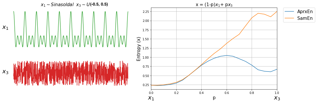
Sample entropy was proposed as the improved version of Approximate entropy, here we can compare both with a small simulation.
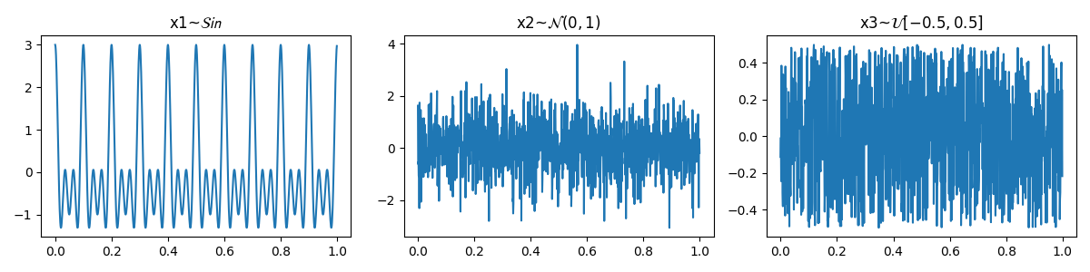
To compare Sample Entropy and Approximate Entropy, let’s first create three signals with expected entropy values.
\[ \begin{align}\begin{aligned}x1 \thicksim \mathcal{Sin}(10,20,30)\\x2 \thicksim \mathcal{N}(0,1)\\x3 \thicksim \mathcal{U}(-0.5,0.5)\end{aligned}\end{align} \]
\(x1\) is a sinusodal signal with three frequency components, \(x2\) drawn from Normal distribution \(\mathcal{N}(0,1)\) and \(x3\) from Uniform Distribuation values ranges from -0.5, 0.5.
import numpy as np
import matplotlib.pyplot as plt
import spkit as sp

fs = 1000
t = np.arange(1000)/fs
x1 = np.cos(2*np.pi*10*t)+np.cos(2*np.pi*30*t)+np.cos(2*np.pi*20*t)
np.random.seed(1)
x2 = np.random.randn(1000)
x3 = np.random.rand(1000)-0.5
Let’s compute Sample and Aprroximate Entropy of these three signals.
Hx1_apx = sp.entropy_approx(x1,m=3,r=0.2*np.std(x1))
Hx2_apx = sp.entropy_approx(x2,m=3,r=0.2*np.std(x2))
Hx3_apx = sp.entropy_approx(x3,m=3,r=0.2*np.std(x3))

print(Hx1_apx, Hx2_apx, Hx3_apx)

Hx1_sae = sp.entropy_sample(x1,m=3,r=0.2*np.std(x1))
Hx2_sae = sp.entropy_sample(x2,m=3,r=0.2*np.std(x2))
Hx3_sae = sp.entropy_sample(x3,m=3,r=0.2*np.std(x3))
print(Hx1_sae, Hx2_sae, Hx3_sae)
Comparing the entropy values, it can be seen, they are as expected.
x (signal) |
Approximate Entropy |
Sample Entropy |
|---|---|---|
x1 ~ \(\mathcal{Sin}(10,20,30)\) |
0.23429 |
0.23462 |
x2 ~ \(\mathcal{N}(0,1)\) |
0.59213 |
2.19315 |
x3 ~ \(\mathcal{U}(-0.5, 0.5)\) |
0.67204 |
2.24992 |
Compare execution time
import time
tt1 = []
for _ in range(5):
  start = time.process_time()
  sp.entropy_approx(x1,m=3,r=0.2*np.std(x1))
  tt1.append(time.process_time() - start)
  print(time.process_time() - start)


tt2 = []
for _ in range(5):
  start = time.process_time()
  sp.entropy_sample(x1,m=3,r=0.2*np.std(x1))
  tt2.append(time.process_time() - start)
  print(time.process_time() - start)


print(f'Approx Entropy:\t {np.mean(tt1)} \t {np.std(tt1)}')
print(f'Sample Entropy:\t {np.mean(tt2)} \t {np.std(tt2)}')
Approximate and Sample Entropy : Time¶ Entropy fun
mean
sd
Approximate Entropy
3.11875
0.06139
Sample Entropy
0.1625
0.0159
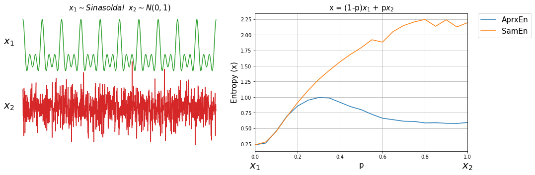
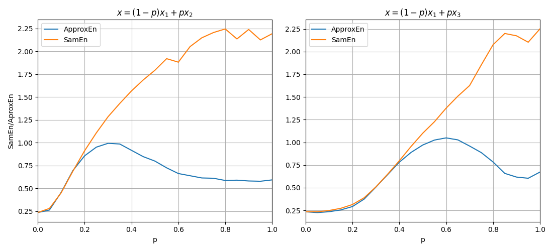
Now, lets compute both entropy values by varies a degree of noise in a signal. This can be done by using a linear combination of x1 and x2, or x1 and x3.
ApSmEn1 = []
ApSmEn2 = []
SD = []

for i,p in enumerate(np.arange(0,1+0.04,0.05)):
    sp.utils.ProgBar(i,22)

    x41 = x1*(1-p) + p*x2
    aprEn = sp.entropy_approx(x41,m=3,r=0.2*np.std(x41))
    smEn  = sp.entropy_sample(x41,m=3,r=0.2*np.std(x41))
    ApSmEn1.append([p,aprEn,smEn])


    x42 = x1*(1-p) + p*x3
    aprEn = sp.entropy_approx(x42,m=3,r=0.2*np.std(x42))
    smEn  = sp.entropy_sample(x42,m=3,r=0.2*np.std(x42))
    ApSmEn2.append([p,aprEn,smEn])

    SD.append([p,0.2*np.std(x41),0.2*np.std(x42)])

ApSmEn1 = np.array(ApSmEn1)
ApSmEn2 = np.array(ApSmEn2)
SD = np.array(SD)
1.1.16. Spectral Entropy & Permutation Entropy
#TODO
References
Click for more details