Note
Go to the end to download the full example code or to run this example in your browser via JupyterLite or Binder
Ramanujan Filter Banks Example
import numpy as np
import matplotlib.pyplot as plt
from mpl_toolkits.axes_grid1 import make_axes_locatable
import spkit as sp


# # Example with Ramanujan Filter Banks
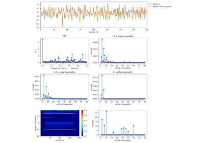
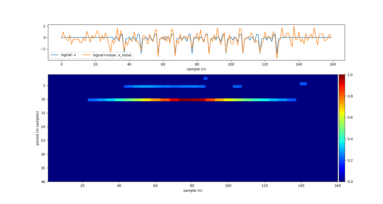
Signal with period 10 and SNR = 0
period = 10
SNR = 0
x0 = np.zeros(30)
x1 = np.random.randn(period)
x1 = np.tile(x1,10)
x = np.r_[x0,x1,x0]
x_noise = sp.add_noise(x,snr_db=SNR)
# ## Period Estimation
Pmax = 40 # Maximum period expected
Rcq = 10 # Number of repeats in each Ramanujan filter
Rav = 2 # Number of repeats in each averaging filter
Th = 0.2 # Threshold zero out the output
y,FR, FA = sp.ramanujan_filter(x_noise,Pmax=Pmax, Rcq=Rcq, Rav=Rav, Th=Th,return_filters=True)
fig, ax = plt.subplots(2,1,figsize=(15,8),height_ratios=[1, 3])
ax[0].plot(x,label='signal: x')
ax[0].plot(x_noise, label='signal+noise: x_noise')
ax[0].set_xlabel('sample (n)')
ax[0].legend(ncol=2)
divider = make_axes_locatable(ax[1])
cax = divider.append_axes('right', size='2%', pad=0.05)
im = ax[1].imshow(y.T,aspect='auto',cmap='jet',extent=[1,len(x_noise),Pmax,1])
#ax[1].set_colorbar(im)
ax[1].set_xlabel('sample (n)')
ax[1].set_ylabel('period (in samples)')
fig.colorbar(im, cax=cax, orientation='vertical')
plt.show()
plt.figure()
plt.stem(np.arange(1,y.shape[1]+1),np.sum(y,0))
plt.xlabel('period (in samples)')
plt.ylabel('strength')
plt.show()
print('top 10 periods: ',np.argsort(np.sum(y,0))[::-1][:10]+1)
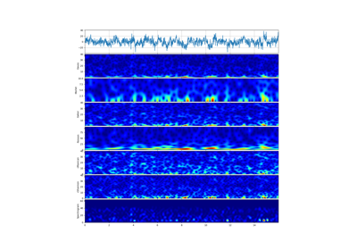
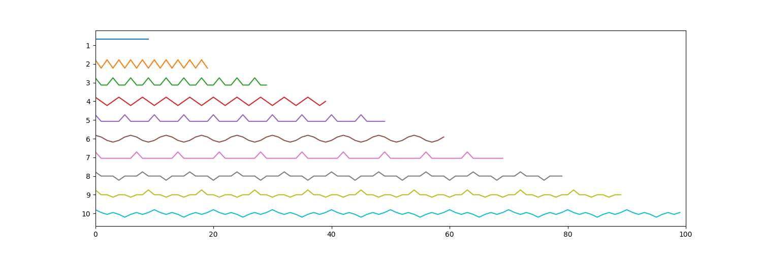
# ## Ramanujan filter
plt.figure(figsize=(15,5))
for i in range(10):
plt.plot(FR[i] - i*1)
plt.xlim([0,len(FR[i])])
plt.yticks(-np.arange(10), np.arange(1,10+1))
plt.show()
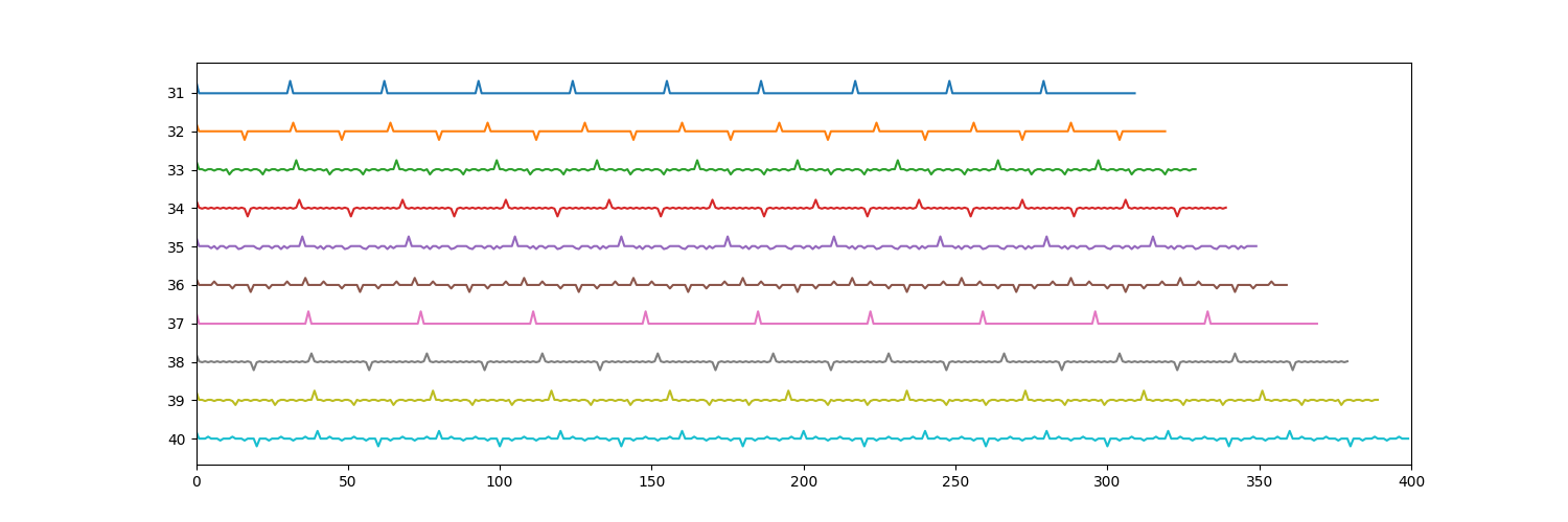
# ### 30-40 filters
plt.figure(figsize=(15,5))
for i in range(30,40):
plt.plot(FR[i] - (i-30)*1)
plt.xlim([0,len(FR[i])])
plt.yticks(-np.arange(10), np.arange(1,10+1)+30)
plt.show()
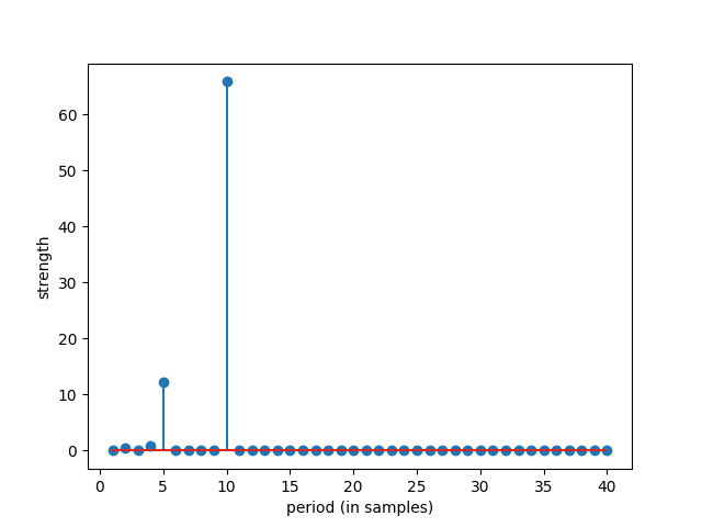
top 10 periods: [10 5 4 2 12 18 17 16 15 14]
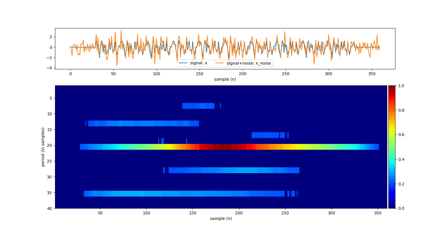
Period Estimation from specific range of period
# ## Signal with period 30

period = 30
SNR = 0

x0 = np.zeros(30)
x1 = np.random.randn(period)
x1 = np.tile(x1,10)
x  = np.r_[x0,x1,x0]

x_noise = sp.add_noise(x,snr_db=SNR)


# ## Period estimation with range


y,Plist = sp.ramanujan_filter_prange(x=x_noise,Pmin=20,Pmax=40, Rcq=10, Rav=2, thr=0.2,return_filters=False)

fig, ax = plt.subplots(2,1,figsize=(15,8),height_ratios=[1, 3])
ax[0].plot(x,label='signal: x')
ax[0].plot(x_noise, label='signal+noise: x_noise')
ax[0].set_xlabel('sample (n)')
ax[0].legend(ncol=2)

divider = make_axes_locatable(ax[1])
cax = divider.append_axes('right', size='2%', pad=0.05)

im = ax[1].imshow(y.T,aspect='auto',cmap='jet',extent=[1,len(x_noise),Pmax,1])
#ax[1].set_colorbar(im)
ax[1].set_xlabel('sample (n)')
ax[1].set_ylabel('period (in samples)')
fig.colorbar(im, cax=cax, orientation='vertical')
plt.show()

Penrgy = np.sum(y,0)

plt.figure()
plt.stem(Plist,Penrgy)
plt.xlabel('period (in samples)')
plt.ylabel('strength')
plt.show()

print('top 10 periods: ',Plist[np.argsort(Penrgy)[::-1]][:10])
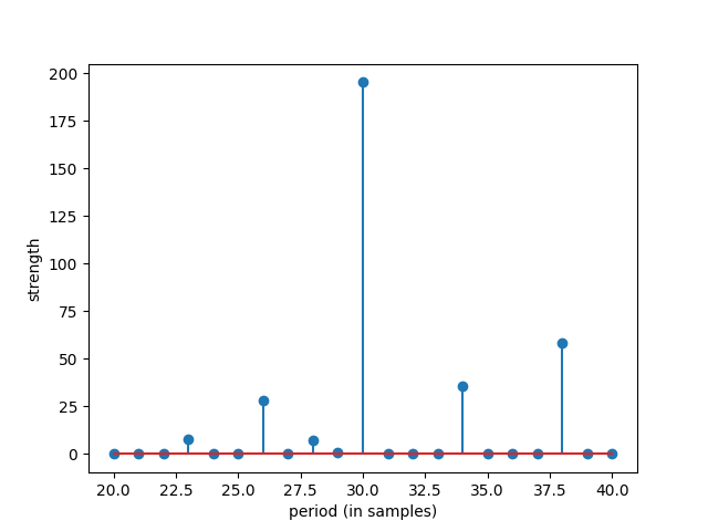
top 10 periods: [30 38 34 26 23 28 29 21 22 24]
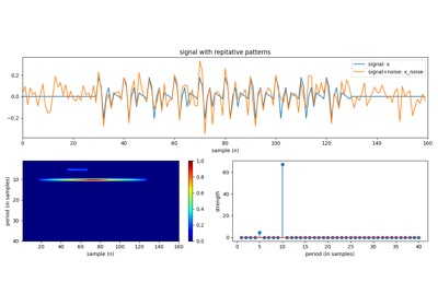
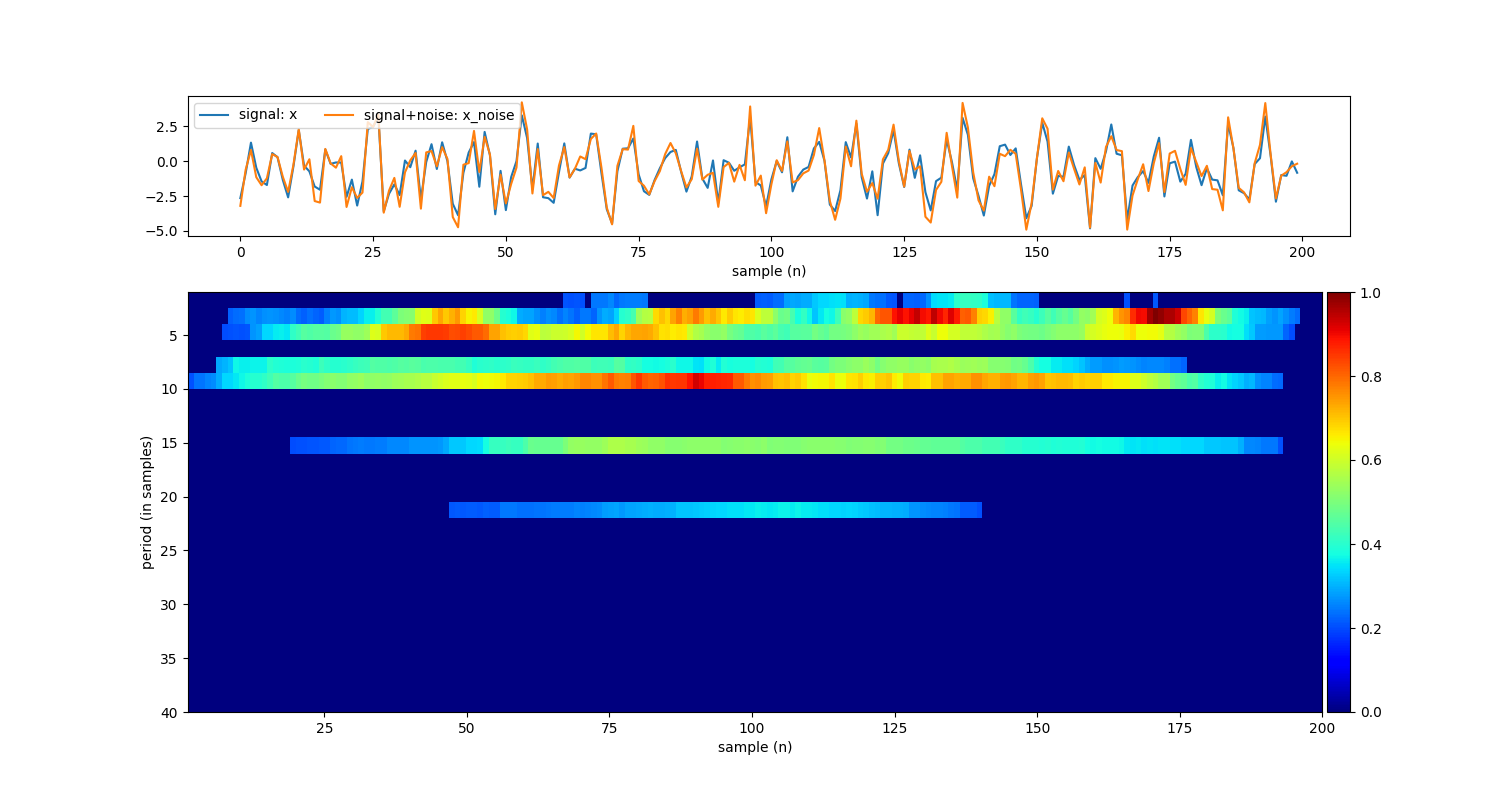
Multiple Periods
periods    = [10,14,18]
signal_length = 200
SNR = 10

x = np.zeros(signal_length)

for period in periods:
    x_temp  = np.random.randn(period)
    x_temp  = np.tile(x_temp,int(np.ceil(signal_length/period)))
    x_temp  = x_temp[:signal_length]
    x += x_temp

x_noise = sp.add_noise(x,snr_db=SNR)


y,Plist = sp.ramanujan_filter_prange(x=x_noise,Pmin=5,Pmax=30, Rcq=10, Rav=2, thr=0.2,return_filters=False)

fig, ax = plt.subplots(2,1,figsize=(15,8),height_ratios=[1, 3])
ax[0].plot(x,label='signal: x')
ax[0].plot(x_noise, label='signal+noise: x_noise')
ax[0].set_xlabel('sample (n)')
ax[0].legend(ncol=2)

divider = make_axes_locatable(ax[1])
cax = divider.append_axes('right', size='2%', pad=0.05)

im = ax[1].imshow(y.T,aspect='auto',cmap='jet',extent=[1,len(x_noise),Pmax,1])
#ax[1].set_colorbar(im)
ax[1].set_xlabel('sample (n)')
ax[1].set_ylabel('period (in samples)')
fig.colorbar(im, cax=cax, orientation='vertical')
plt.show()

Penrgy = np.sum(y,0)
plt.figure()
plt.stem(Plist,Penrgy)
plt.xlabel('period (in samples)')
plt.ylabel('strength')
plt.show()

print('top 10 periods: ',Plist[np.argsort(Penrgy)[::-1]][:10])
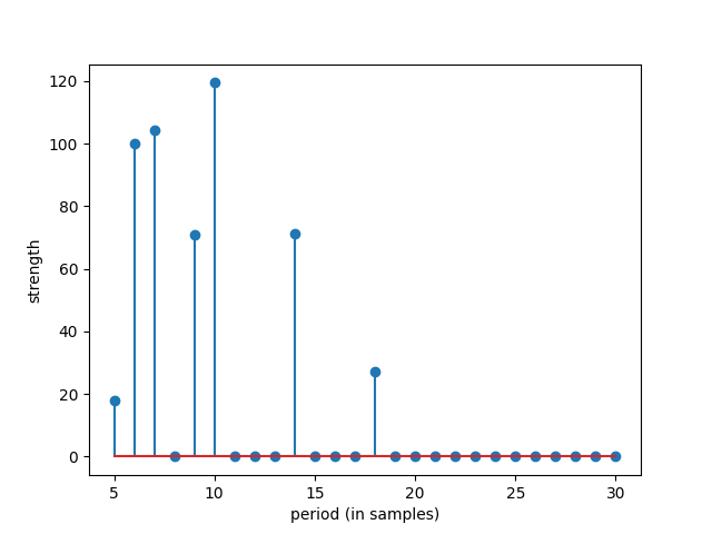
top 10 periods: [10 7 6 14 9 18 5 16 8 11]
Total running time of the script: (0 minutes 0.705 seconds)
Related examples