spkit.ml.LogisticRegression

class spkit.ml.LogisticRegression(alpha=0.01, lambd=0, polyfit=False, degree=3, FeatureNormalize=False, penalty='l2', tol=0.01, rho=0.9, C=1.0, fit_intercept=True)

Logistic Regression

fitting a linear model

For binary

\[y_p = sigmoid(X \times W + b)\]

For multiclass

\[y_p = softmax(X \times W + b)\]

Optimizing \(W\) and \(b\), using gradient decent and regularize with ‘l1’,’l2’ or ‘elastic-net’ penalty

Parameters:

fit_intercept: bool, default=True

• if use intercept (b) to fit, if false, b = 0

alpha: scalar,

• Learning rate, the rate to update the weights at each iteration

penalty: str, {‘l1’, ‘l2, ‘elastic-net’, ‘none’}, default=’l2’

• regularization:

  • ‘l1’ –> lambd*|W|,

  • ‘l2’ –> lambd*|W|**2

  • ‘elastic-net’ - lambd*(rho*|W|^2 + (1-rho)*|W|))

lambdscalar, default =0

• penalty value ()

rhoscalar

• used for elastic-net penalty

tolfloat, default=1e-4

• Tolerance for stopping criteria.

polyfit: bool, default=False

• if polynomial features to be used,

degree: int,default=2

• degree of polynomial features, used if polyfit is true,

FeatureNormalize: bool, default=False

• if true, before fitting and after polyfit, features are normalized

  and computed mean and std is saved to be used while prediction

Attributes:

nclass: ndarray of shape (n_classes, )

• A list of class labels known to the classifier.

W: ndarray of shape (1, n_features) or (n_classes, n_features)

• Coefficient of the features in the decision function.

b: intercept weight

• intercept weight

See also

NaiveBayes, ClassificationTree, RegressionTree

Examples

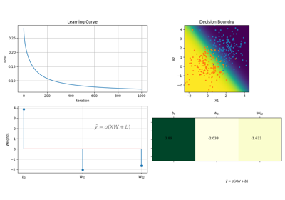
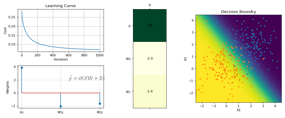
#sp.ml.LogisticRegression
import numpy as np
import matplotlib.pyplot as plt
import spkit as sp
from spkit.ml import LogisticRegression
#--------------- Binary Class ------
N = 300
np.random.seed(1)
X = np.random.randn(N,2)
y = np.random.randint(0,2,N)
y.sort()
X[y==0,:]+=2 # just creating classes a little far
print(X.shape, y.shape)
#(300, 2) (300,)
model = LogisticRegression(alpha=0.1)
model.fit(X,y,max_itr=1000)
yp  = model.predict(X)
ypr = model.predict_proba(X)
print('Accuracy : ',np.mean(yp==y))
print('Loss     : ',model.Loss(y,ypr))
#Accuracy :  0.96
#Loss     :  0.07046678918014998
fig = plt.figure(figsize=(12,5))
gs = fig.add_gridspec(2,3)
ax1 = fig.add_subplot(gs[0, 0])
ax2 = fig.add_subplot(gs[1, 0])
ax3 = fig.add_subplot(gs[:, 1])
ax4 = fig.add_subplot(gs[:, 2])
model.plot_Lcurve(ax=ax1)
model.plot_weights(ax=ax2)
model.plot_weights2(ax=ax3)
model.plot_boundries(X,y,alphaP=1,ax=ax4)
plt.tight_layout()
plt.show()

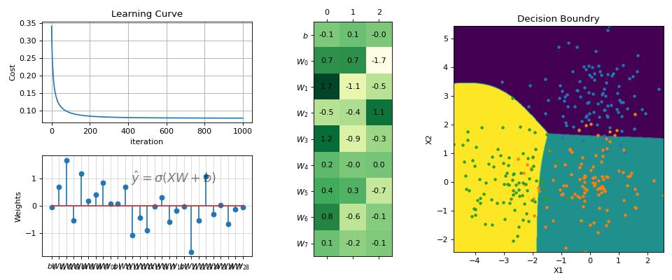
# ------- Multi Class ------
N =300
X = np.random.randn(N,2)
y = np.random.randint(0,3,N)
y.sort()
X[y==0,1]+=3
X[y==2,0]-=3
print(X.shape, y.shape)
#(300, 2) (300,)
model = LogisticRegression(alpha=0.1,polyfit=True,degree=3,lambd=0,FeatureNormalize=True)
model.fit(X,y,max_itr=1000)
yp  = model.predict(X)
ypr = model.predict_proba(X)
print('Accuracy : ',np.mean(yp==y))
print('Loss     : ',model.Loss(model.oneHot(y),ypr))
#Accuracy :  0.8833333333333333
#Loss     :  0.08365012491975303
fig = plt.figure(figsize=(12,5))
gs = fig.add_gridspec(2,3)
ax1 = fig.add_subplot(gs[0, 0])
ax2 = fig.add_subplot(gs[1, 0])
ax3 = fig.add_subplot(gs[:, 1])
ax4 = fig.add_subplot(gs[:, 2])
model.plot_Lcurve(ax=ax1)
model.plot_weights(ax=ax2)
model.plot_weights2(ax=ax3)
model.plot_boundries(X,y,alphaP=1,ax=ax4)
plt.tight_layout()
plt.show()

Methods

Loss(y, yp)	Loss Function
Normalize(X)	Normalization
PolyFeature(X[, degree])	Polynomial Feature Extrations
fit(X, y[, max_itr, verbose, printAt, warm])	Fitting the model
getWeights()	Get Weights
getWeightsAsList()	Get Weights
oneHot(y)	Convert y to One hot vector
plot_Lcurve([ax])	Plot Learning Curve
plot_boundries(X, y[, ax, density, ...])	Plot Boundaries
plot_weights([ax, show_eq, fontsize, alpha])	Plot Weights
plot_weights2([ax, fontsize, grid])	Plot Weights as matrix
predict(X)	Prediction
predict_proba(X)	Predict probability
regularization(W)	Regularization
sigmoid(z)	Sigmoid function
softmax(z)	Softmax function

Loss(y, yp)

Loss Function

Normalize(X)

Normalization

PolyFeature(X, degree=2)

Polynomial Feature Extrations

Parameters:

X: 2d-array (n,nf)

• n samples, nf features

degree: int, default=2

• degree of polynomials to comput

• for degree of 2, f1**2, f2**2 … is computed and f1*f2*f3 ..

Returns:

Xp: 2d-array (n,mf)

• new feature matrix with polynomial features

fit(X, y, max_itr=-1, verbose=0, printAt=100, warm=True)

Fitting the model

Parameters:

Xndarray

• (N,nf),

yndarray of int (N,)

• y \(\in\) [0,1,…]

max_itr: int,

• number of iteration, if -1, set to 10000

verbose: int,0,

• silent, 1, minimum verbosity, 11, debug mode

warm: bool,

• if false, weights will be reinitialize, else, last trained weights will be used

getWeights()

Get Weights

getWeightsAsList()

Get Weights

Returns:

bW: 2d-array

• weights : [b, W]

Wl: list of str

• label of weights

oneHot(y)

Convert y to One hot vector

plot_Lcurve(ax=None)

Plot Learning Curve

plot_boundries(X, y, ax=None, density=500, hardbound=False, alphaP=1, alphaB=1)

Plot Boundaries

Only for 2D dataset

Parameters:

X: features matirx

y: labels

ax: plt axis, default None

density: pixel density for plot

hardbound: bool, default=False

• if True, then final classification decisions are used

• else classification probalities are used

plot_weights(ax=None, show_eq=True, fontsize=16, alpha=0.5)

Plot Weights

Parameters:

ax: default None,

• axis to plot, if not provided, then fig, ax = plt.subplots()

show_eq: bool, default=True

• if true, equation is written on plot as text

fontsize: fontsize of equation

alpha: alpha for equation text

plot_weights2(ax=None, fontsize=10, grid=True)

Plot Weights as matrix

predict(X)

Prediction

predict_proba(X)

Predict probability

regularization(W)

Regularization

sigmoid(z)

Sigmoid function

softmax(z)

Softmax function

Examples using spkit.ml.LogisticRegression

Logistic Regression - Visualisation

Logistic Regression - Visualisation