spkit.friedrichs_mollifier_kernel
- spkit.friedrichs_mollifier_kernel(window_size, s=1, p=2, r=0.999)
Mollifier: Kurt Otto Friedrichs
Mollifier: Kurt Otto Friedrichs
Generalized function
\[f(x) = exp(-s/(1-|x|**p)) for |x|<1, x \in [-r, r]\]Convolving with a mollifier, signals’s sharp features are smoothed, while still remaining close to the original nonsmooth (generalized) signals.
Intuitively, given a function which is rather irregular, by convolving it with a mollifier the function gets “mollified”.
This function is infinitely differentiable, non analytic with vanishing derivative for |x| = 1, can be therefore used as mollifier as described in [1]. This is a positive and symmetric mollifier.[15]
- Parameters:
- window_size: int, size of windows
- s: scaler, s>0, default=1,
Spread of the middle width, heigher the value of s, narrower the width
- p: scaler, p>0, default=2,
Order of flateness of the peak at the top,
p=2, smoother, p=1, triangulare type
Higher it is, more flat the peak.
- r: float, 0<r<1, default=0.999,
it is used to compute x = [-r, r]
recommonded to keep it r=0.999
- Returns:
- ker_mol: mollifier kernel
See also
gaussian_kernelGaussian Kernel
References
Examples
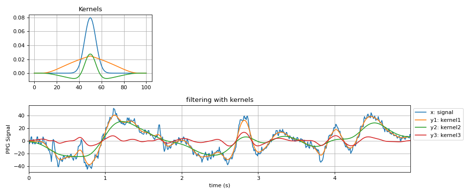
#sp.friedrichs_mollifier_kernel
import numpy as np
import matplotlib.pyplot as plt
import spkit as sp
x,fs = sp.data.ppg_sample(sample=1)
x = x[:int(fs*5)]
x = x - x.mean()
t = np.arange(len(x))/fs
kernel1 = sp.gaussian_kernel(window_length=101,sigma_scale=10)
kernel2 = sp.friedrichs_mollifier_kernel(window_size=101,s=1,p=1)
kernel3 = (kernel1 - kernel2)/2
y1 = sp.filter_with_kernel(x.copy(),kernel=kernel1)
y2 = sp.filter_with_kernel(x.copy(),kernel=kernel2)
y3 = sp.filter_with_kernel(x.copy(),kernel=kernel3)
plt.figure(figsize=(12,5))
plt.subplot(212)
plt.plot(t,x,label='x: signal')
plt.plot(t,y1,label='y1: kernel1')
plt.plot(t,y2,label='y2: kernel2')
plt.plot(t,y3,label='y3: kernel3')
plt.xlim([t[0],t[-1]])
plt.xlabel('time (s)')
plt.ylabel('PPG Signal')
plt.grid()
plt.legend(bbox_to_anchor=(1,1))
plt.title('filtering with kernels')
plt.subplot(231)
plt.plot(kernel1,label='kernel1')
plt.plot(kernel2,label='kernel2')
plt.plot(kernel3,label='kernel3')
plt.title('Kernels')
plt.grid()
plt.tight_layout()
plt.show()