spkit.cwt.ShannonWave
- spkit.cwt.ShannonWave(t, f, f0=0.75, fw=0.5)
Complex Shannon Wavelet
Generate Wavelet functions to be used for analysis
\[ \begin{align}\begin{aligned}\psi(t) &= Sinc(t/2) \cdot e^{-2j\pi f_0t}\\\psi(w) &= \prod \left( \frac{w-w_0}{\pi} \right)\end{aligned}\end{align} \]where
\(\prod (x) = 1\) if \(x \leq 0.5\), 0 else
\(w = 2\pi f\) and \(w_0 = 2\pi f_0\)
- Parameters:
- t: 1d array,
time span array corresponding to signal for analysis,
must be centered at 0
- f: 1d array,
frquency array for wavelet analysis
- f0: scalar or array, default = 3/4
array of center frquencies for wavelets,
0.1*np.arange(10)
- fw: scalar or array, default 0.5
BandWidth each wavelet, , could be an array (not suggeestive)
- Returns:
- wttime-domain wavelet(s)
- wffrequency-domain wavelet(s)
See also
Notes
It is efficient and easy to use
ScalogramCWTwith wType==’cShannon’ code:XW,S = ScalogramCWT(x,t,fs=fs,wType='cShannon',PlotPSD=True)
References
wikipedia - https://en.wikipedia.org/wiki/Shannon_wavelet
Examples
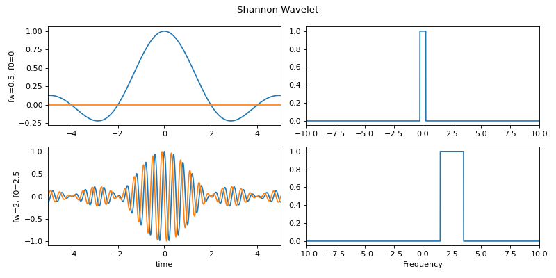
#sp.cwt.ShannonWave
import numpy as np
import matplotlib.pyplot as plt
import spkit as sp
fs = 100                              #sampling frequency
t = np.linspace(-5,5,fs*10+1)         #time
f = np.linspace(-10,10,2*len(t)-1)    #frequency range
#f = np.linspace(-fs//2,fs//2,2*len(t))   #frequency range
wt1,wf1 = sp.cwt.ShannonWave(t,f,f0=0,fw=0.5)
wt2,wf2 = sp.cwt.ShannonWave(t,f,f0=2.5,fw=2)
plt.figure(figsize=(10,5))
plt.subplot(221)
plt.plot(t,wt1.T.real,label='real')
plt.plot(t,wt1.T.imag,'-',label='image')
plt.xlim(t[0],t[-1])
plt.ylabel('fw=0.5, f0=0')
plt.subplot(222)
plt.plot(f,abs(wf1.T))
plt.xlim(f[0],f[-1])
plt.subplot(223)
plt.plot(t,wt2.T.real,label='real')
plt.plot(t,wt2.T.imag,'-',label='image')
plt.xlim(t[0],t[-1])
plt.xlabel('time')
plt.ylabel('fw=2, f0=2.5')
plt.subplot(224)
plt.plot(f,abs(wf2.T))
plt.xlim(f[0],f[-1])
plt.xlabel('Frequency')
plt.suptitle('Shannon Wavelet')
plt.tight_layout()
plt.show()