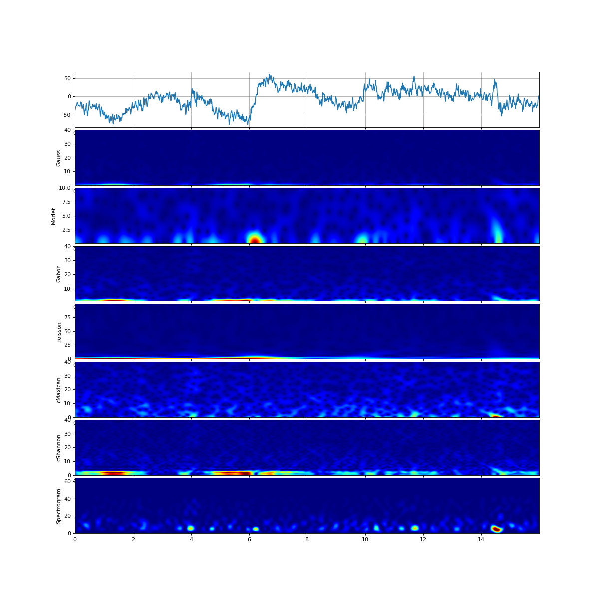
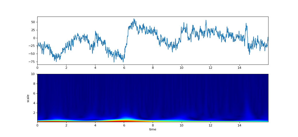
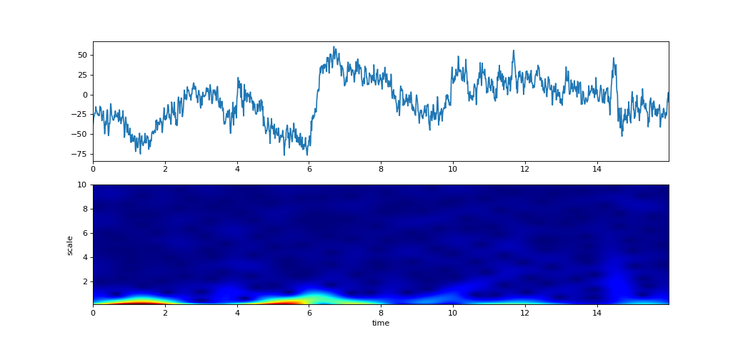
`spkit.cwt`.ScalogramCWT¶

spkit.cwt.ScalogramCWT(x, t, wType='Gauss', fs=128, PlotPSD=False, PlotW=False, fftMeth=True, interpolation='sinc', **Parameters)¶

Scalogram using Continues Wavelet Transform

Compute scalogram using Continues Wavelet Transform for wavelet type (wType) and given scale range

Parameters:

x: array-like,

input signal,

t: array-like

time array corresponding to x, same length as x

fs: int,

sampling rate

PlotPSD: bool, default=False

if True, plot Scalogram

PlotWbool, default=False

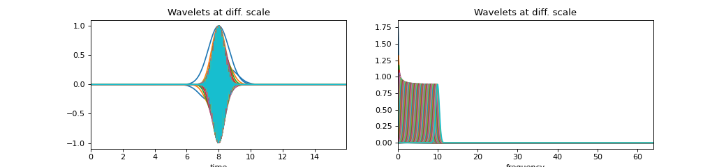
if True, plot wavelets in time and frequecy with different scalling version

fftMeth:bool, default=True

if True, FFT method is used, else convolution method is used. FFT method is faster.

interpolation: str, or None,

interpolation while ploting Scalogram. Only used for plotting

Parameters for different wavelet functions

Common Parameters for all the Wavelet functions

farray

array of frequency range to be analysed, e.g. np.linspace(-10,10,2*N-1), where N = len(x)
if None, frequency range of signal is considered from -fs/2 to fs/2
(fs/n1*(np.arange(n1)-n1/2))

A list of wavelets will be generated for each value of scale (e.g. f0, sigma, n etc)

wType: {‘Gauss’,’Morlet’,’Gabor’,’Poisson’,’cMaxican’,’cShannon’}

Type of Complext Wavelet Function
lower case str is acceptable, and a few common names are mapped to them too
‘Gauss’, ‘gauss’, ‘gaussian’ are same
‘cMaxican’, ‘maxican’, ‘cmaxican’ are same
‘cShannon’ ‘shannon’ are same

1. Gauss: (wType ==’Gauss’)

f0 = array of center frquencies for wavelets, default: np.linspace(0.1,10,100) [scale value] Q = float or array of q-factor for each wavelet, e.g. 0.5 (default) or np.linspace(0.1,5,100)

: if array, should be of same size as f0

t0 = float=0, time shift of wavelet, or phase shift in frquency, Not suggeestive to change

2. For Morlet: (wType ==’Morlet’)

sig = array of sigma values for morlet wavelet, default: np.linspace(0.1,10,100) [scale value] fw = array of frequency range, e.g. np.linspace(-10,10,2*N-1), where N = len(x) ref: https://en.wikipedia.org/wiki/Morlet_wavelet

3. For Gabor: (wType ==’Gabor’)

Gauss and Gabor wavelet are essentially same f0 = array of center frquencies for wavelets, default: np.linspace(1,40,100) [scale value] a = float, oscillation parameter, default 0.5,

could be an array (not suggeestive), similar to Gauss, e.g np.linspace(0.1,1,100) or np.logspace(0.001,0.5,100)

t0 = float=0, time shift of wavelet, or phase shift in frquency. Not suggeestive to change

4. For Poisson: (wType==’Poisson’)

n = array of intergers, default np.arange(100), [scale value] method = 1,2,3, different implementation of Poisson funtion, default 3 keep the method=3, other methods are under development and not exactly compatibile with framework yet,

ref: https://en.wikipedia.org/wiki/Poisson_wavelet

5. For Complex MaxicanHat: (wType==’cMaxican’)

f0 = array of center frquencies for wavelets, default: np.linspace(1,40,100) [scale value] a = float, oscillation parameter, default 1.0, could be an array (not suggeestive)

ref: https://en.wikipedia.org/wiki/Complex_Mexican_hat_wavelet

6. For Complex Shannon: (wType==’cShannon’)

f0 = array of center frquencies for wavelets, default: 0.1*np.arange(10) [scale value], fw = BandWidth each wavelet, default 0.5, could be an array (not suggeestive)

ref: https://en.wikipedia.org/wiki/Shannon_wavelet

Returns:

XW: Complex-valued matrix of time-scale - Scalogram, with shape (len(S), len(x)). scale vs time
Sscale values

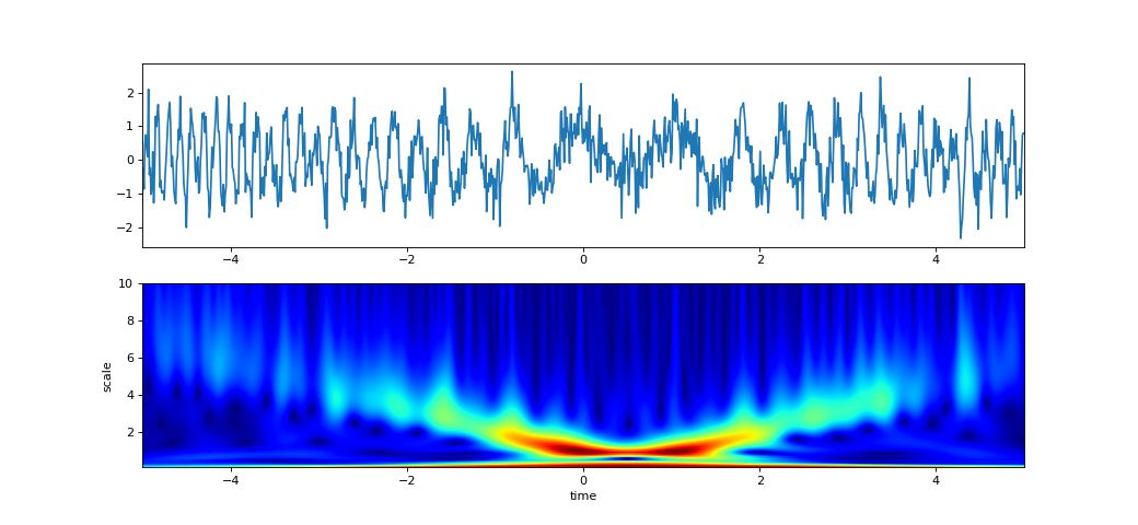
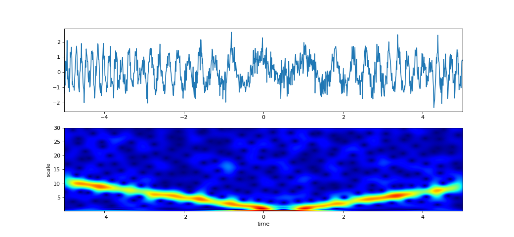
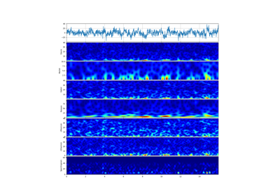
Examples

import numpy as np
import matplotlib.pyplot as plt
from spkit.cwt import ScalogramCWT

# Example 1 - EEG Signal
import spkit as sp
from spkit.cwt import compare_cwt_example
x,fs = sp.data.eeg_sample_1ch(ch=0)
t = np.arange(len(x))/fs
print(x.shape, t.shape)
compare_cwt_example(x,t,fs=fs)

# Example 2.1 - different wavelets
XW,S = ScalogramCWT(x,t,fs=fs,wType='Gauss',PlotPSD=True)

# Example 2.2 - set scale values and number of points
nS = 100
f0 = np.linspace(0.1,10,nS) # range of scale values - frquency
Q  = np.linspace(0.1,5,nS)  # different q-factor for each scale value
# Q = 0.5
XW,S = ScalogramCWT(x,t,fs=fs,wType='Gauss',PlotPSD=True,f0=f0,Q=Q)

# Example 2.3  - plot scalled wavelets too
XW,S = ScalogramCWT(x,t,fs=fs,wType='Gauss',PlotPSD=True,PlotW=True,f0=f0,Q=Q)

# Example 3
t = np.linspace(-5, 5, 10*100)
x = (np.sin(2*np.pi*0.75*t*(1-t) + 2.1) + 0.1*np.sin(2*np.pi*1.25*t + 1) + 0.18*np.cos(2*np.pi*3.85*t))
xn = x + np.random.randn(len(t)) * 0.5
XW,S = ScalogramCWT(xn,t,fs=100,wType='Gauss',PlotPSD=True)

# Example 4
f0 = np.linspace(0.1,30,100)
Q  = np.linspace(0.1,5,100) # or = 0.5
XW,S = ScalogramCWT(xn,t,fs=128,wType='Gauss',PlotPSD=True,f0=f0,Q=Q)