spkit.cwt.PoissonWave

spkit.cwt.PoissonWave(t, f=1, n=1, method=3)

Poisson Wavelet

Type 1 (n): Method=1

$$\begin{array}{r}\begin{array}{rl}\psi (t)& =\left(\frac{t-n}{n!}\right)t^{n-1}{e}^{-t}\\ \psi (w)& =\frac{-jw}{(1+jw{)}^{n+1}}\end{array}\end{array}$$

where Admiddibility const $C_{\psi }=\frac{1}{n}$ and $w=2\pi f$

Type 2: Method=2

$$\begin{array}{r}\begin{array}{rl}\psi (t)& =\frac{1}{\pi }\frac{1-t^2}{(1+t^2{)}^2}\\ \psi (t)& =p(t)+\frac{d}{dt}p(t)\\ \psi (w)& =|w|e^{-|w|}\end{array}\end{array}$$

where

$$\begin{array}{r}\begin{array}{rl}p(t)& =\frac{1}{\pi }\frac{1}{1+t^2}\\ w& =2\pi f\end{array}\end{array}$$

Type 3 (n): Method=3

$$\begin{array}{r}\begin{array}{rl}\psi (t)& =\frac{1}{2\pi }(1-jt{)}^{-(n+1)}\\ \psi (w)& =\frac{1}{\mathrm{\Gamma }n+1}{w}^n{e}^{-w}u(w)\end{array}\end{array}$$

where

Unit step function

$$\begin{array}{r}\begin{array}{rl}u(w)& =1\text{ if }w>=0\text{else }0\\ w& =2\pi f\end{array}\end{array}$$

Parameters:

t: 1d array,

• time span array corresponding to signal for analysis,

• must be centered at 0

f: 1d array,

• frquency array for wavelet analysis

n: int, array, default=1

• array of integers

• np.arange(100), [scale value]

method: {1,2,3}, default=3

• method to select the type of Poisson wavelet computations method = 1,2,3, different implementation of Poisson funtion, default 3 keep the method=3, other methods are under development and not exactly compatibile with framework yet,

Returns:

wttime-domain wavelet(s)

wffrequency-domain wavelet(s)

See also

ScalogramCWT

Notes

Method 3 produces more stable results It is efficient and easy to use ScalogramCWT with wType==’Poisson’ code:

XW,S = ScalogramCWT(x,t,fs=fs,wType='Poisson',method = 3,PlotPSD=True)

References

• wikipedia - https://en.wikipedia.org/wiki/Poisson_wavelet

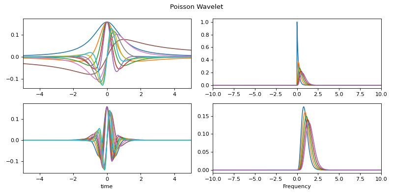
Examples

#sp.cwt.PoissonWave
import numpy as np
import matplotlib.pyplot as plt
import spkit as sp
fs = 100                              #sampling frequency
t = np.linspace(-5,5,fs*10+1)         #time
f = np.linspace(-10,10,2*len(t)-1)    #frequency range
#f = np.linspace(-fs//2,fs//2,2*len(t))   #frequency range
n1 = np.arange(5)
n2 = np.arange(5,10)
wt1,wf1 = sp.cwt.PoissonWave(t,f=f,n=n1,method=3)
wt2,wf2 = sp.cwt.PoissonWave(t,f=f,n=n2,method=3)

plt.figure(figsize=(10,5))
plt.subplot(221)
plt.plot(t,wt1.T.real,label='real')
plt.plot(t,wt1.T.imag,'-',label='image')
plt.xlim(t[0],t[-1])
plt.subplot(222)
plt.plot(f,abs(wf1.T))
plt.xlim(f[0],f[-1])
plt.subplot(223)
plt.plot(t,wt2.T.real,label='real')
plt.plot(t,wt2.T.imag,'-',label='image')
plt.xlim(t[0],t[-1])
plt.xlabel('time')
plt.subplot(224)
plt.plot(f,abs(wf2.T))
plt.xlim(f[0],f[-1])
plt.xlabel('Frequency')
plt.suptitle('Poisson Wavelet')
plt.tight_layout()
plt.show()