spkit.cwt.MorlateWave
- spkit.cwt.MorlateWave(t, f=1, sig=1)
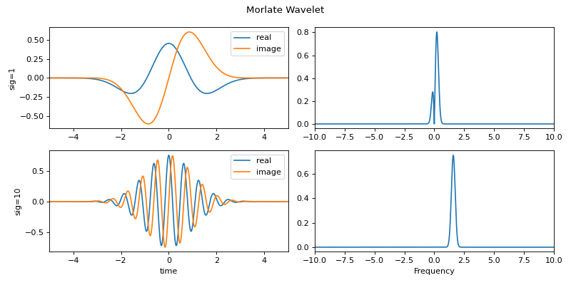
Morlate Wavelet
Generate time and frequency domain Morlate wavelet functions
\[ \begin{align}\begin{aligned}\psi(t) &= C_{\sigma}\pi^{-0.25} e^{-0.5t^2} \left(e^{j\sigma t}-K_{\sigma} \right)\\\psi(w) &= C_{\sigma}\pi^{-0.25} \left(e^{-0.5(\sigma-w)^2} -K_{\sigma}e^{-0.5w^2} \right)\end{aligned}\end{align} \]where
\[ \begin{align}\begin{aligned}C_{\sigma} &= \left(1+ e^{-\sigma^{2}} - 2e^{-\frac{3}{4}\sigma^{2}} \right)^{-0.5}\\K_{\sigma} &=e^{-0.5\sigma^{2}} w &= 2\pi f\end{aligned}\end{align} \]- Parameters:
- t: 1d array,
time span array corresponding to signal for analysis,
must be centered at 0
- sig: scalar or array
array of sigma values for morlet wavelet, default=1 [scale value]
np.linspace(0.1,10,100)
- f: array
array of frequency range, e.g. np.linspace(-10,10,2*N-1), where N = len(x) or len(t)
- Returns:
- wttime-domain wavelet(s)
- wffrequency-domain wavelet(s)
See also
Notes
It is efficient and easy to use
ScalogramCWTwith wType==’Morlet’ code:XW,S = ScalogramCWT(x,t,fs=fs,wType='Morlet',PlotPSD=True)
References
wikipedia - https://en.wikipedia.org/wiki/Morlet_wavelet
Examples
#sp.cwt.MorlateWave
import numpy as np
import matplotlib.pyplot as plt
import spkit as sp
fs = 100                              #sampling frequency
t = np.linspace(-5,5,fs*10+1)         #time
f = np.linspace(-10,10,2*len(t)-1)    #frequency range
sig1  = 1    #np.linspace(0.1,10,100)
sig2  = 10
wt1,wf1 = sp.cwt.MorlateWave(t,f,sig=sig1)
wt2,wf2 = sp.cwt.MorlateWave(t,f,sig=sig2)
plt.figure(figsize=(10,5))
plt.subplot(221)
plt.plot(t,wt1.T.real,label='real')
plt.plot(t,wt1.T.imag,'-',label='image')
plt.xlim(t[0],t[-1])
#plt.xlabel('time')
plt.ylabel(f'sig={sig1}')
plt.legend()
plt.subplot(222)
plt.plot(f,abs(wf1.T))
plt.xlim(f[0],f[-1])
plt.xlim(-10,10)
plt.subplot(223)
plt.plot(t,wt2.T.real,label='real')
plt.plot(t,wt2.T.imag,'-',label='image')
plt.xlim(t[0],t[-1])
plt.xlabel('time')
plt.ylabel(f'sig={sig2}')
plt.legend()
plt.subplot(224)
plt.plot(f,abs(wf2.T))
plt.xlim(f[0],f[-1])
plt.xlim(-10,10)
plt.xlabel('Frequency')
#plt.legend()
plt.suptitle('Morlate Wavelet')
plt.tight_layout()
plt.show()