3.1. Continues Wavelet Transform

>>> import numpy as np
>>> import matplotlib.pyplot as plt

>>> import spkit
>>> print('spkit-version ', spkit.__version__)
>>> import spkit as sp
>>> x,fs = sp.load_data.eegSample_1ch()
>>> t = np.arange(len(x))/fs
>>> sp.cwt.compare_cwt_example(x,t,fs=fs)

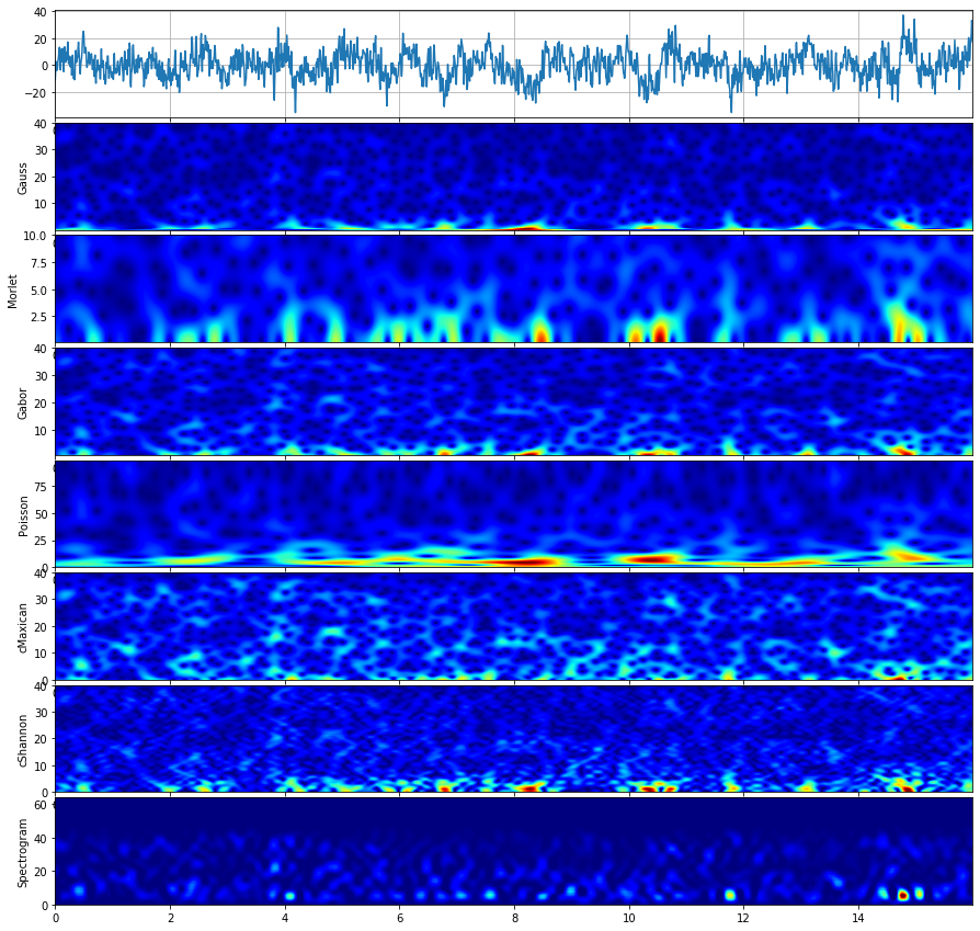
3.1.1. Gauss wavelet

The Gauss Wavelet function in time and frequency domain are defined as \(\psi(t)\) and \(\psi(f)\) as below;

\[\begin{split}\psi(t) &= e^{-a(t-t_0)^{2}} \cdot e^{-2\pi jf_0(t-t_0)}\\ \psi(f) &= \sqrt{\pi/a}\left( e^{-2\pi jft_0}\cdot e^{-\pi^{2}((f-f_0)^{2})/a}\right)\end{split}\]

where

\[a = \left( \frac{f_0}{Q} \right)^{2}\]

Parameters for a Gauss wavelet:

• f0 - center frequency

• Q - associated with spread of bandwidth, as a = (f0/Q)^2

>>> XW,S = sp.cwt.ScalogramCWT(x,t,fs=fs,wType='Gauss',PlotPSD=True)

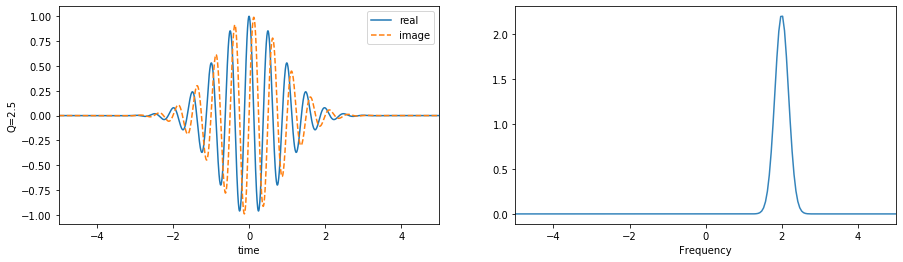
3.1.1.1. Plot wavelet functions

To plot as analysis the wavelet functions

>>> fs = 128                                   #sampling frequency
>>> tx = np.linspace(-5,5,fs*10+1)             #time
>>> fx = np.linspace(-fs//2,fs//2,2*len(tx))   #frequency range
>>> f01 = 2     #np.linspace(0.1,5,2)[:,None]
>>> Q1  = 2.5   #np.linspace(0.1,5,10)[:,None]
>>> wt1,wf1 = sp.cwt.GaussWave(tx,f=fx,f0=f01,Q=Q1)
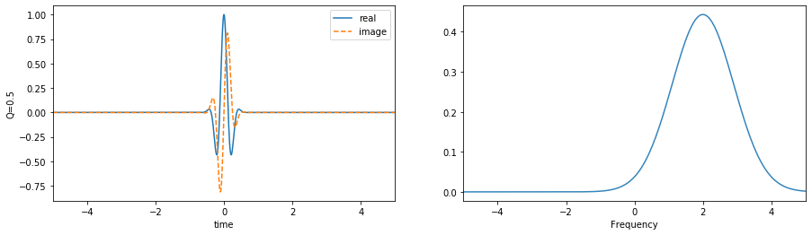
>>> f02 = 2    #np.linspace(0.1,5,2)[:,None]
>>> Q2  = 0.5  #np.linspace(0.1,5,10)[:,None]
>>> wt2,wf2 = sp.cwt.GaussWave(tx,f=fx,f0=f02,Q=Q2)
>>> plt.figure(figsize=(15,4))
>>> plt.subplot(121)
>>> plt.plot(tx,wt1.T.real,label='real')
>>> plt.plot(tx,wt1.T.imag,'--',label='image')
>>> plt.xlim(tx[0],tx[-1])
>>> plt.xlabel('time')
>>> plt.ylabel('Q=2.5')
>>> plt.legend()
>>> plt.subplot(122)
>>> plt.plot(fx,abs(wf1.T), alpha=0.9)
>>> plt.xlim(fx[0],fx[-1])
>>> plt.xlim(-5,5)
>>> plt.xlabel('Frequency')
>>> plt.show()
>>> plt.figure(figsize=(15,4))
>>> plt.subplot(121)
>>> plt.plot(tx,wt2.T.real,label='real')
>>> plt.plot(tx,wt2.T.imag,'--',label='image')
>>> plt.xlim(tx[0],tx[-1])
>>> plt.xlabel('time')
>>> plt.ylabel('Q=0.5')
>>> plt.legend()
>>> plt.subplot(122)
>>> plt.plot(fx,abs(wf2.T), alpha=0.9)
>>> plt.xlim(fx[0],fx[-1])
>>> plt.xlim(-5,5)
>>> plt.xlabel('Frequency')
>>> plt.show()

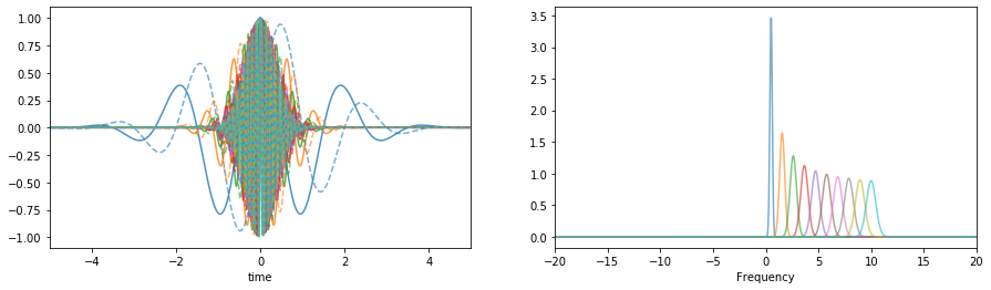
3.1.1.2. With a range of scale parameters

Changing the range of scale

>>> f0 = np.linspace(0.5,10,10)[:,None]
>>> Q  = np.linspace(1,5,10)[:,None]
>>> #Q  = 1
>>> wt,wf = sp.cwt.GaussWave(tx,f=fx,f0=f0,Q=Q)
>>> plt.figure(figsize=(15,4))
>>> plt.subplot(121)
>>> plt.plot(tx,wt.T.real, alpha=0.8)
>>> plt.plot(tx,wt.T.imag,'--', alpha=0.6)
>>> plt.xlim(tx[0],tx[-1])
>>> plt.xlabel('time')
>>> plt.subplot(122)
>>> plt.plot(fx,abs(wf.T), alpha=0.6)
>>> plt.xlim(fx[0],fx[-1])
>>> plt.xlim(-20,20)
>>> plt.xlabel('Frequency')
>>> plt.show()

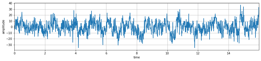
3.1.1.3. Signal Analysis - EEG

Example with EEG Signal

>>> x,fs = sp.load_data.eegSample_1ch()
>>> t = np.arange(len(x))/fs
>>> print('shape ',x.shape, t.shape)
>>> plt.figure(figsize=(15,3))
>>> plt.plot(t,x)
>>> plt.xlabel('time')
>>> plt.ylabel('amplitude')
>>> plt.xlim(t[0],t[-1])
>>> plt.grid()
>>> plt.show()

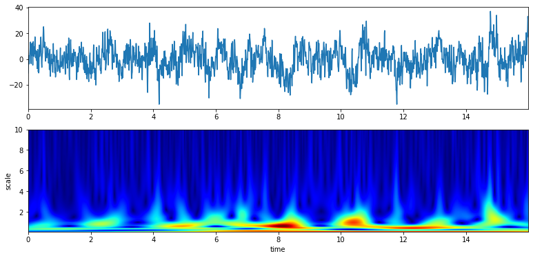
3.1.1.4. Scalogram with default parameters

With default setting of f0 and Q

• f0 = np.linspace(0.1,10,100)

• Q = 0.5

  >>> XW,S = sp.cwt.ScalogramCWT(x,t,fs=fs,wType='Gauss',PlotPSD=True)
  

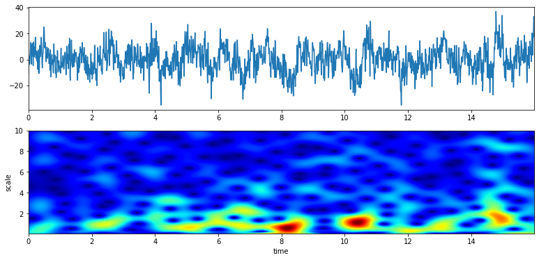
3.1.1.5. With a range of frequency and Q

From 0.1 to 10 Hz of analysis range and 100 points

>>> f0 = np.linspace(0.1,10,100)
>>> Q  = np.linspace(0.1,5,100)
>>> XW,S = sp.cwt.ScalogramCWT(x,t,fs=fs,wType='Gauss',PlotPSD=True,f0=f0,Q=Q)

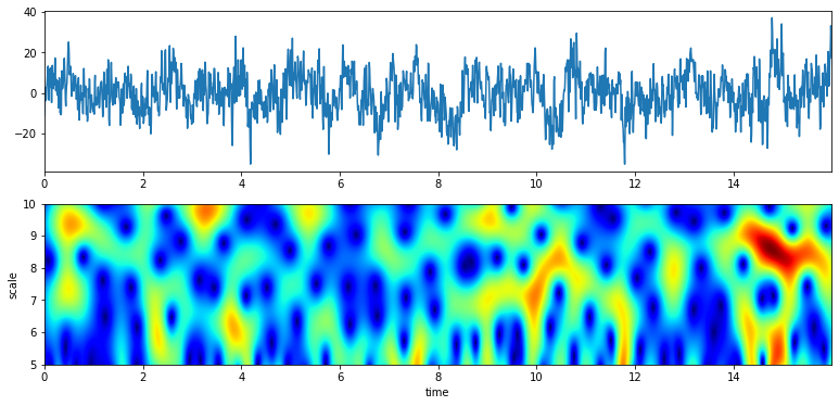
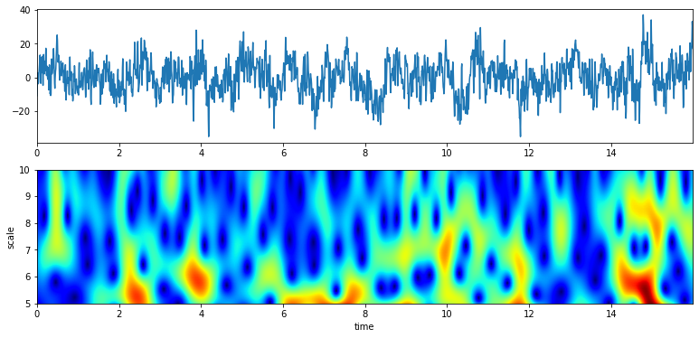
From 5 to 10 Hz of analysis range and 100 points

>>> f0 = np.linspace(5,10,100)
>>> Q  = np.linspace(1,4,100)
>>> XW,S = sp.cwt.ScalogramCWT(x,t,fs=fs,wType='Gauss',PlotPSD=True,f0=f0,Q=Q)

With constant Q

>>> f0 = np.linspace(5,10,100)
>>> Q  = 2
>>> XW,S = sp.cwt.ScalogramCWT(x,t,fs=fs,wType='Gauss',PlotPSD=True,f0=f0,Q=Q)

From 12 to 24 Hz

>>> f0 = np.linspace(12,24,100)
>>> Q  = 4
>>> XW,S = sp.cwt.ScalogramCWT(x,t,fs=fs,wType='Gauss',PlotPSD=True,f0=f0,Q=Q)

3.1.1.6. With a plot of analysis wavelets

>>> f0 = np.linspace(12,24,100)
>>> Q  = 4
>>> XW,S = sp.cwt.ScalogramCWT(x,t,fs=fs,wType='Gauss',PlotPSD=True,PlotW=True, f0=f0,Q=Q)

#TODO Speech/Audio Signal

3.1.1.7. Speech

#TODO

3.1.1.8. Audio

#TODO

3.1.2. Morlet wavelet

#TODO

The Morlet Wavelet function in time and frequency domain are defined as \(\psi(t)\) and \(\psi(f)\) as below;

\[\begin{split}\psi(t) &= C_{\sigma}\pi^{-0.25} e^{-0.5t^2} \left(e^{j\sigma t}-K_{\sigma} \right)\\ \psi(w) &= C_{\sigma}\pi^{-0.25} \left(e^{-0.5(\sigma-w)^2} -K_{\sigma}e^{-0.5w^2} \right)\end{split}\]

where

\[\begin{split}C_{\sigma} &= \left(1+ e^{-\sigma^{2}} - 2e^{-\frac{3}{4}\sigma^{2}} \right)^{-0.5}\\ K_{\sigma} &=e^{-0.5\sigma^{2}}\\ w &= 2\pi f\end{split}\]

>>> XW,S = sp.cwt.ScalogramCWT(x,t,fs=fs,wType='Morlet',PlotPSD=True)

3.1.3. Gabor wavelet

#TODO

The Gabor Wavelet function (technically same as Gaussian) in time and frequency domain are defined as \(\psi(t)\) and \(\psi(f)\) as below;

\[\begin{split}\psi(t) &= e^{-(t-t_0)^2/a^2}e^{-jf_0(t-t_0)}\\ \psi(f) &= e^{-((f-f_0)a)^2}e^{-jt_0(f-f_0)}\end{split}\]

where

\(a\) is oscilation rate and \(f_0\) is center frequency

>>> XW,S = sp.cwt.ScalogramCWT(x,t,fs=fs,wType='Gabor',PlotPSD=True)

3.1.4. Poisson wavelet

Poisson wavelet is defined by positive integers ($n$), unlike other, and associated with Poisson probability distribution

The Poisson Wavelet function in time and frequency domain are defined as \(\psi(t)\) and \(\psi(f)\) as below;

3.1.4.1. #Type 1 (n)

\[\begin{split}\psi(t) &= \left(\frac{t-n}{n!}\right)t^{n-1} e^{-t}\\ \psi(w) &= \frac{-jw}{(1+jw)^{n+1}}\end{split}\]

where

Admiddibility const \(C_{\psi} =\frac{1}{n}\) and \(w = 2\pi f\)

>>> XW,S = sp.cwt.ScalogramCWT(x,t,fs=fs,wType='Poisson',method = 1,PlotPSD=True)

3.1.4.2. #Type 2

\[ \begin{align}\begin{aligned}\psi(t) &= \frac{1}{\pi} \frac{1-t^2}{(1+t^2)^2}\\\psi(t) &= p(t) + \frac{d}{dt}p(t)\\\psi(w) &= |w|e^{-|w|}\end{aligned}\end{align} \]

where

\[ \begin{align}\begin{aligned}p(t) &=\frac{1}{\pi}\frac{1}{1+t^2}\\w &= 2\pi f\end{aligned}\end{align} \]

>>> XW,S = sp.cwt.ScalogramCWT(x,t,fs=fs,,wType='Poisson',method = 2,PlotPSD=True)

3.1.4.3. #Type 3 (n)

\[ \begin{align}\begin{aligned}\psi(t) &= \frac{1}{2\pi}(1-jt)^{-(n+1)}\\\psi(w) &= \frac{1}{\Gamma{n+1}}w^{n}e^{-w}u(w)\end{aligned}\end{align} \]

where .

\[ \begin{align}\begin{aligned}\text{unit step function }\quad u(w) &=1 \quad \text{ if $w>=0$ }\quad \text{else } 0\\w &= 2\pi f\end{aligned}\end{align} \]

>>> XW,S = sp.cwt.ScalogramCWT(x,t,fs=fs,wType='Poisson',method = 3,PlotPSD=True)

#TODO

3.1.5. Maxican wavelet

Complex Mexican hat wavelet is derived from the conventional Mexican hat wavelet. It is a low-oscillation wavelet which is modulated by a complex exponential function with frequency \(f_0\) Ref..

The Maxican Wavelet function in time and frequency domain are defined as \(\psi(t)\) and \(\psi(f)\) as below;

\[\begin{split}\psi(t) &= \frac{2}{\sqrt{3}} \pi^{-\frac{1}{4}}\left(\sqrt{\pi}(1-t^2)e^{-\frac{1}{2}t^2} - \left(\sqrt{2}jt + \sqrt{\pi}erf\left[\frac{j}{\sqrt{2}}t \right] (1-t^2)e^{-\frac{1}{2}t^2}\right)\right)e^{-2\pi jf_0 t}\\\\ \psi(w) &= 2\sqrt{\frac{2}{3}}\pi^{-1/4}(w-w_0)^2e^{-\frac{1}{2} (w-w_0)^2} \quad \text{ if $w\ge 0$,}\quad \text{ 0 else}\end{split}\]

where \(w = 2\pi f\) and \(w_0 = 2\pi f_0\)

>>> XW,S = sp.cwt.ScalogramCWT(x,t,fs=fs,wType='cMaxican',PlotPSD=True)

#TODO

3.1.6. Shannon wavelet

Complex Shannon wavelet is the most simplified wavelet function, exploiting Sinc function by modulating with sinusoidal, which results in an ideal bandpass filter. Real Shannon wavelet is modulated by only a cos function Ref.

The Shannon Wavelet function in time and frequency domain are defined as \(\psi(t)\) and \(\psi(f)\) as below;

\[\begin{split}\psi(t) &= Sinc(t/2) \cdot e^{-2j\pi f_0t}\\ \psi(w) &= \prod \left( \frac{w-w_0}{\pi} \right)\end{split}\]

where

where \(\prod (x) = 1\) if \(x \leq 0.5\), 0 else and \(w = 2\pi f\) and \(w_0 = 2\pi f_0\)

>>> XW,S = sp.cwt.ScalogramCWT(x,t,fs=fs,wType='cShannon',PlotPSD=True)

#TODO