spkit.A_law
- spkit.A_law(x, A=255, companding=True)
A-Law for companding and expanding (Non-linear mapping)
A-Law for companding and expanding - A-Law is one of the ways to map gaussian, or laplacian distribuated signal to uniformly distributed one - for companding - smaller amplitude values are stretched (since they have high-probabilty)
and large amplitutde values are compressed (since they have low probabiltity)
for expending - it reverts the mapping
for -1 ≤ x ≤ 1 and 1 < A
- Companding:
- \[ \begin{align}\begin{aligned}y(n) &= sign(x)* \frac{A|x|}{(1 + log(A))} if |x|<1/A\\ &= sign(x)* \frac{((1 + log(A|x|))} {(1 + log(A)))} else\end{aligned}\end{align} \]
expanding:
\[ \begin{align}\begin{aligned}y(n) = sign(x)* \frac{|x|(1+log(A))} {A} if |x|<1/(1+log(A))\\ = sign(x)* \frac{(exp(-1 + |x|(1+log(A))))} {A} else\end{aligned}\end{align} \]An alternative to μ-Law
The μ-law algorithm provides a slightly larger dynamic range than the A-law at the cost of worse proportional distortions for small signals.
- Parameters:
- x - 1d (or nd) array of signal, must be -1 ≤ x ≤ 1
- A - scalar (1≤A) - factor for companding-expanding mapping
1: identity function, higher value of A will stretch and compress more
- companding: (bool) - if True, companding is applied, else expanding
- Returns:
- y - mapped output of same shape as x
See also
A_lawA-Law for companding and expanding
References
wikipedia - https://en.wikipedia.org/wiki/A-law_algorithm
Examples
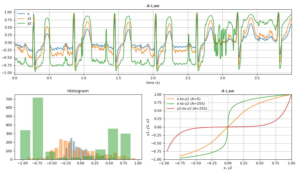
#sp.A_law
import numpy as np
import matplotlib.pyplot as plt
import spkit as sp
x,fs,_ = sp.data.ecg_sample_12leads(sample=3)
x = x[1000:3000,0]
x = x/(np.abs(x).max()*1.01)
x = x - np.mean(x)
x = x/(np.abs(x).max()*1.01)
t = np.arange(len(x))/fs
y1 = sp.A_law(x.copy(),A=5,companding=True)
y2 = sp.A_law(x.copy(),A=255,companding=True)
x2 = sp.A_law(y2.copy(),A=255,companding=False)
plt.figure(figsize=(12,7))
plt.subplot(211)
plt.plot(t,x,label=f'x')
plt.plot(t,y1,label=f'y1')
plt.plot(t,y2,label=f'y2')
plt.xlim([t[0],t[-1]])
plt.xlabel('time (s)')
plt.legend()
plt.title('$A$-Law')
plt.grid()
plt.subplot(223)
sp.hist_plot(x)
sp.hist_plot(y1)
sp.hist_plot(y2)
plt.title('Histogram')
plt.subplot(224)
idx = np.argsort(x)
plt.plot(x[idx],y1[idx],color='C1',label='x-to-y1 (A=5)')
plt.plot(x[idx],y2[idx],color='C2',label='x-to-y2 (A=255)')
plt.plot(y2[idx],x[idx],color='C3',label='y2-to-x2 (A=255)')
plt.xlim([-1,1])
plt.ylim([-1,1])
plt.xlabel('x, y2')
plt.ylabel('y1, y2, x2')
plt.title(r'$A$-Law')
plt.grid()
plt.legend()
plt.tight_layout()
plt.show()