Machine Learning

New Updates

Decision Tree - View Notebooks

• Version: 0.0.9:

• Analysing the performance measure of trained tree at different depth - with ONE-TIME Training ONLY

• Optimize the depth of tree

• Shrink the trained tree with optimal depth

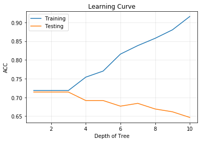
• Plot the Learning Curve

• Classification: Compute the probability and counts of label at a leaf for given example sample

• Regression: Compute the standard deviation and number of training samples at a leaf for given example sample

• Version: 0.0.6: Works with catogorical features without converting them into binary vector

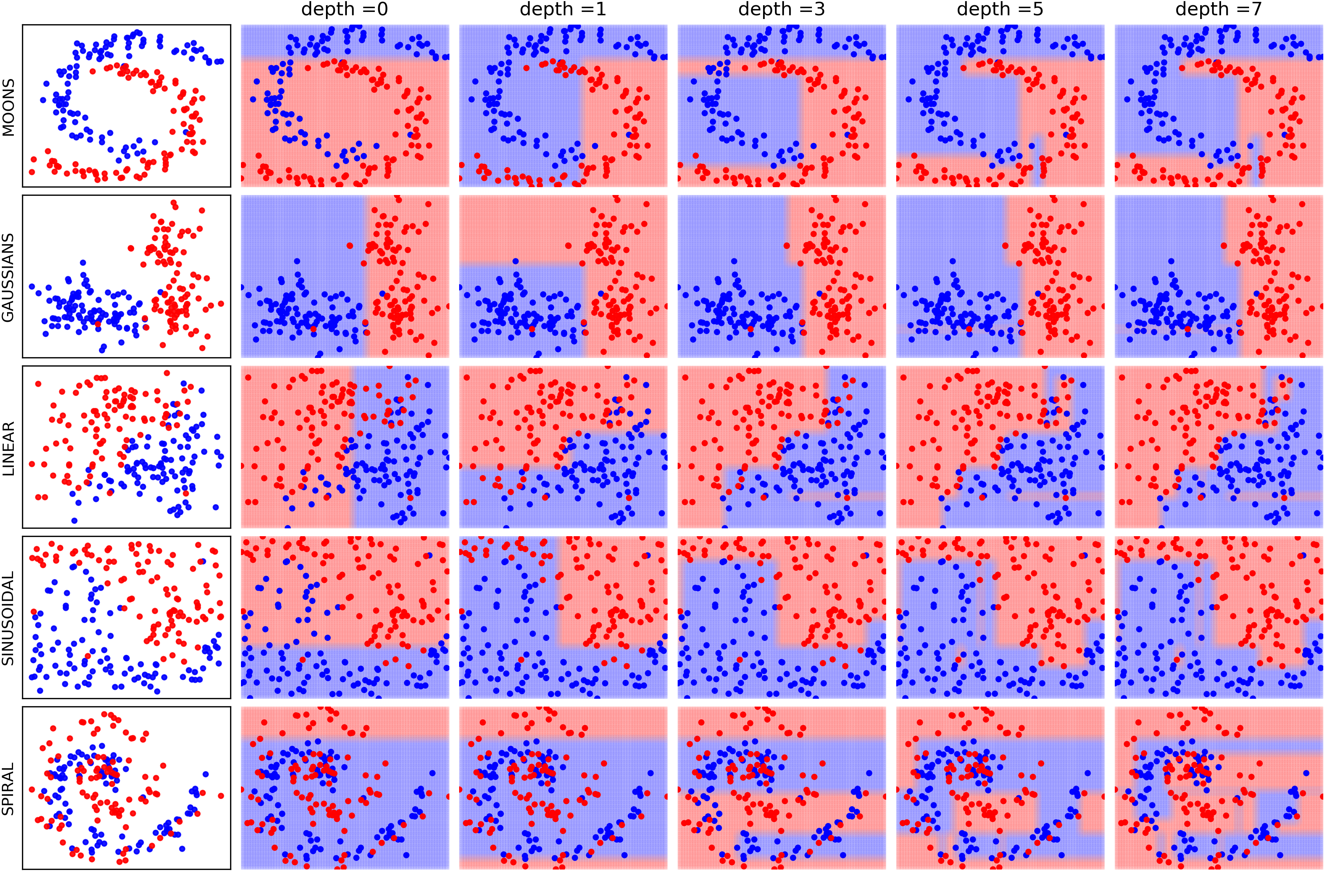
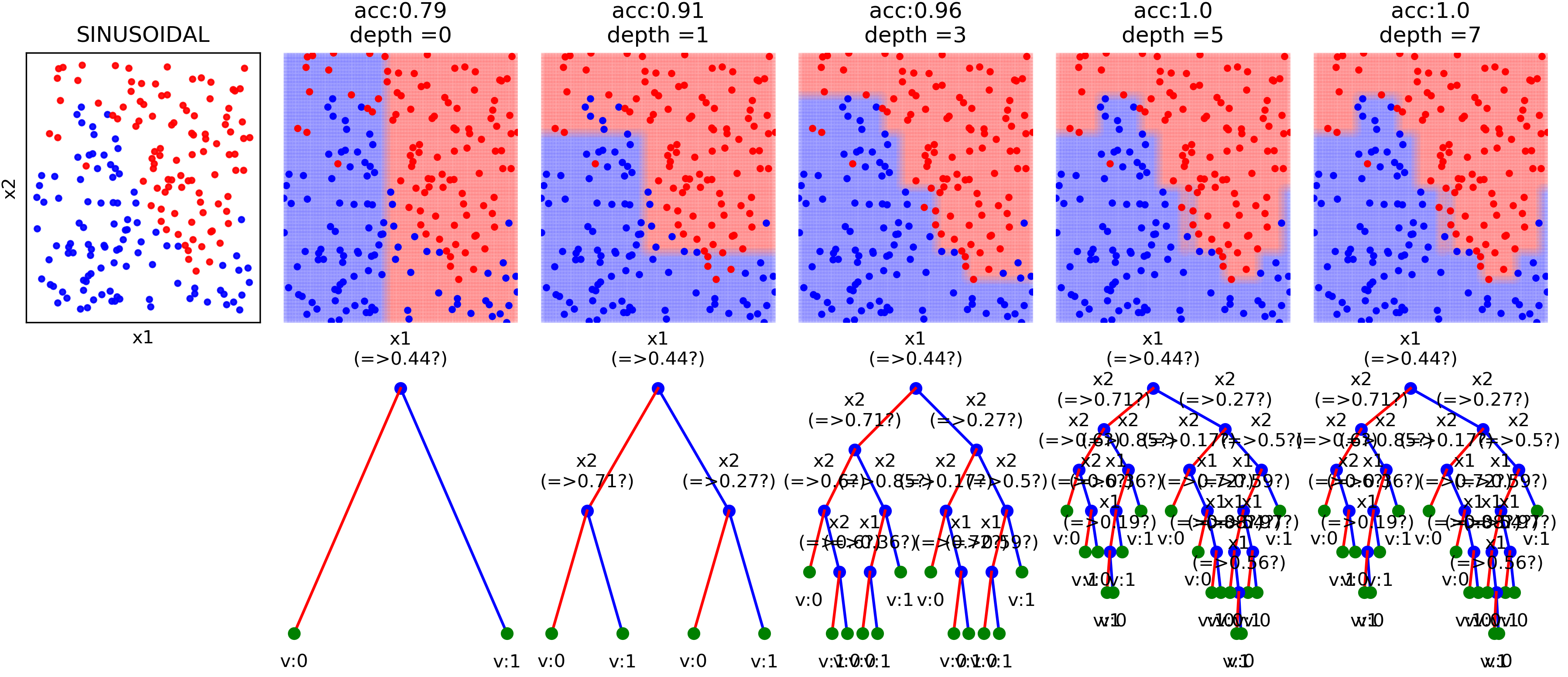
• Version: 0.0.5: Toy examples to understand the effect of incresing max_depth of Decision Tree

Logistic Regression

View more examples in Notebooks

Binary Class

import numpy as np
import matplotlib.pyplot as plt

import spkit
print(spkit.__version__)
0.0.9

from spkit.ml import LogisticRegression

# Generate data
N = 300
np.random.seed(1)
X = np.random.randn(N,2)
y = np.random.randint(0,2,N)
y.sort()

X[y==0,:]+=2 # just creating classes a little far
print(X.shape, y.shape)
plt.plot(X[y==0,0],X[y==0,1],'.b')
plt.plot(X[y==1,0],X[y==1,1],'.r')
plt.show()


clf = LogisticRegression(alpha=0.1)
print(clf)
clf.fit(X,y,max_itr=1000)
yp  = clf.predict(X)
ypr = clf.predict_proba(X)
print('Accuracy : ',np.mean(yp==y))
print('Loss     : ',clf.Loss(y,ypr))

plt.figure(figsize=(12,7))
ax1 = plt.subplot(221)
clf.plot_Lcurve(ax=ax1)
ax2 = plt.subplot(222)
clf.plot_boundries(X,y,ax=ax2)

ax3 = plt.subplot(223)
clf.plot_weights(ax=ax3)
ax4 = plt.subplot(224)
clf.plot_weights2(ax=ax4,grid=False)

Multi Class - with polynomial features

N =300
X = np.random.randn(N,2)
y = np.random.randint(0,3,N)
y.sort()

X[y==0,1]+=3
X[y==2,0]-=3
print(X.shape, y.shape)

plt.plot(X[y==0,0],X[y==0,1],'.b')
plt.plot(X[y==1,0],X[y==1,1],'.r')
plt.plot(X[y==2,0],X[y==2,1],'.g')
plt.show()

clf = LogisticRegression(alpha=0.1,polyfit=True,degree=3,lambd=0,FeatureNormalize=True)
clf.fit(X,y,max_itr=1000)
yp  = clf.predict(X)
ypr = clf.predict_proba(X)
print(clf)
print('')
print('Accuracy : ',np.mean(yp==y))
print('Loss     : ',clf.Loss(clf.oneHot(y),ypr))


plt.figure(figsize=(15,7))
ax1 = plt.subplot(221)
clf.plot_Lcurve(ax=ax1)
ax2 = plt.subplot(222)
clf.plot_boundries(X,y,ax=ax2)

ax3 = plt.subplot(223)
clf.plot_weights(ax=ax3)
ax4 = plt.subplot(224)
clf.plot_weights2(ax=ax4,grid=True)

---

Naive Bayes

View more examples in Notebooks

import numpy as np
import matplotlib.pyplot as plt

#for dataset and splitting
from sklearn import datasets
from sklearn.model_selection import train_test_split


from spkit.ml import NaiveBayes

#Data
data = datasets.load_iris()
X = data.data
y = data.target

Xt,Xs,yt,ys = train_test_split(X,y,test_size=0.3)

print('Data Shape::',Xt.shape,yt.shape,Xs.shape,ys.shape)

#Fitting
clf = NaiveBayes()
clf.fit(Xt,yt)

#Prediction
ytp = clf.predict(Xt)
ysp = clf.predict(Xs)

print('Training Accuracy : ',np.mean(ytp==yt))
print('Testing  Accuracy : ',np.mean(ysp==ys))


#Probabilities
ytpr = clf.predict_prob(Xt)
yspr = clf.predict_prob(Xs)
print('\nProbability')
print(ytpr[0])

#parameters
print('\nParameters')
print(clf.parameters)


#Visualising
clf.set_class_labels(data['target_names'])
clf.set_feature_names(data['feature_names'])


fig = plt.figure(figsize=(10,8))
clf.VizPx()

---

Decision Trees

View more examples in Notebooks

Or just execute all the examples online, without installing anything

One example file is

import numpy as np
import matplotlib.pyplot as plt

# Data and Split
from sklearn.model_selection import train_test_split
from sklearn.datasets import load_diabetes

from spkit.ml import ClassificationTree


data = load_diabetes()
X = data.data
y = 1*(data.target>np.mean(data.target))

feature_names = data.feature_names
print(X.shape, y.shape)
Xt,Xs,yt,ys = train_test_split(X,y,test_size =0.3)
print(Xt.shape, Xs.shape,yt.shape, ys.shape)


clf = ClassificationTree(max_depth=7)
clf.fit(Xt,yt,feature_names=feature_names)
ytp = clf.predict(Xt)
ysp = clf.predict(Xs)

ytpr = clf.predict_proba(Xt)[:,1]
yspr = clf.predict_proba(Xs)[:,1]

print('Depth of trained Tree ', clf.getTreeDepth())
print('Accuracy')
print('- Training : ',np.mean(ytp==yt))
print('- Testing  : ',np.mean(ysp==ys))
print('Logloss')
Trloss = -np.mean(yt*np.log(ytpr+1e-10)+(1-yt)*np.log(1-ytpr+1e-10))
Tsloss = -np.mean(ys*np.log(yspr+1e-10)+(1-ys)*np.log(1-yspr+1e-10))
print('- Training : ',Trloss)
print('- Testing  : ',Tsloss)

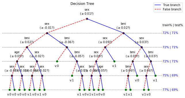
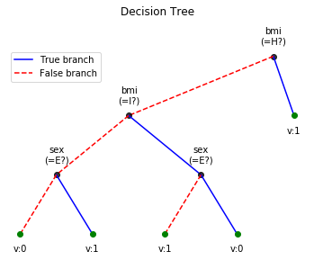
# Plot Tree
plt.figure(figsize=(15,12))
clf.plotTree()

Depth Analysis

View more examples in Notebooks

Plottng tree while training