Information Theory for Real-Valued signals

Updating the documentation …

Entropy of signal with finit set of values is easy to compute, since frequency for each value can be computed, however, for real-valued signal it is a little different, because of infinite set of amplitude values. For which spkit comes handy.

*Following Entropy functions compute entropy based the on the sample distribuation, which by default consider process to be IID (Independent Identical Disstribuation) - which means no temporal dependency.*

*For temporal dependency (non-IID) signals, Spectral, Sample, Aproximate, SVD and Dispersion Entropy functions can be used. Which are discribed below*

Entropy of real-valued signal (~ IID)

**View in Jupyter-Notebook**

---

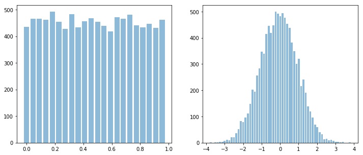
Let’s first start with two signals, (two time series), x with uniform distribution, i.e., x ~ U(), and y with normal distribution, i.e., y ~ N()

import numpy as np
import matplotlib.pyplot as plt
import spkit as sp

x = np.random.rand(10000)
y = np.random.randn(10000)

plt.figure(figsize=(12,5))
plt.subplot(121)
sp.HistPlot(x,show=False)

plt.subplot(122)
sp.HistPlot(y,show=False)
plt.show()

Shannan entropy

Shannon entropy can be computed as follow;

#Shannan entropy
H_x = sp.entropy(x)
H_y = sp.entropy(y)

print('Shannan entropy')
print('Entropy of x: H(x) = ',H_x)
print('Entropy of y: H(y) = ',H_y)

Shannan entropy
Entropy of x: H(x) =  4.4581180171280685
Entropy of y: H(y) =  5.04102391756942

Rényi entropy

Rényi entropy, also known as Collision Entropy. It is generalized form entropy, where shannon entropy is special case with alpha=1.

#Rényi entropy
Hr_x= sp.entropy(x,alpha=2)
Hr_y= sp.entropy(y,alpha=2)
print('Rényi entropy')
print('Entropy of x: H(x) = ',Hr_x)
print('Entropy of y: H(y) = ',Hr_y)

Rényi entropy
Entropy of x: H(x) =  4.456806796146617
Entropy of y: H(y) =  4.828391418226062

Mutual Information

I_xy = sp.mutual_Info(x,y)
print('Mutual Information I(x,y) = ',I_xy)

Joint Entropy H(x,y) =  9.439792556949234

Joint Entropy

H_xy= sp.entropy_joint(x,y)
print('Joint Entropy H(x,y) = ',H_xy)

Mutual Information I(x,y) =  0.05934937774825322

Conditional entropy

H_x1y= sp.entropy_cond(x,y)
H_y1x= sp.entropy_cond(y,x)
print('Conditional Entropy of : H(x|y) = ',H_x1y)
print('Conditional Entropy of : H(y|x) = ',H_y1x)

output:

Conditional Entropy of : H(x|y) = 4.398768639379814 Conditional Entropy of : H(y|x) = 4.9816745398211655

Cross entropy

H_xy_cross= sp.entropy_cross(x,y)
print('Cross Entropy of : H(x,y) = :',H_xy_cross)

Cross Entropy of : H(x,y) = : 11.591688735915701

Kullback–Leibler divergence

D_xy= sp.entropy_kld(x,y)

print('Kullback–Leibler divergence : Dkl(x,y) = :',D_xy)

Kullback–Leibler divergence : Dkl(x,y) = : 4.203058010473213

Entropy of real-valued signal (~ non-IID)

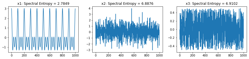
For following section, we will consider three different signals to compare the Entropy,

• x1 ~ \(cos(2\pi 10t)+cos(2\pi 20t)+cos(2\pi 30t)\) - sinasodal signal with three frequency componets

• x2 ~ \(\mathcal{N}(0,1)\) - random gaussian signal with zero mean and sd=1

• x3 ~ \(\mathcal{U}(-0.5, 0.5)\) - random signal with uniform distribution ranges from -0.5 to 0.5, zero mean

Spectral Entropy

Though spectral entropy compute the entropy of frequency components considering that frequency distribution is ~ IID, however, each frequency component has a temporal characteristics, so this is an indirect way to considering the temporal dependency of a signal.

fs = 1000
t = np.arange(1000)/fs
x1 = np.cos(2*np.pi*10*t)+np.cos(2*np.pi*30*t)+np.cos(2*np.pi*20*t)


np.random.seed(1)
x2 = np.random.randn(1000)
x3 = np.random.rand(1000)-0.5


Hx1_se = sp.entropy_spectral(x1,fs=1,method='welch',bining=False,normalize=False)
Hx2_se = sp.entropy_spectral(x2,fs=1,method='welch',bining=False,normalize=False)
Hx3_se = sp.entropy_spectral(x3,fs=1000,method='welch',bining=False,normalize=False)


Hx1_se_n = sp.entropy_spectral(x1,fs=1,method='welch',bining=False,normalize=True)
Hx2_se_n = sp.entropy_spectral(x2,fs=1,method='welch',bining=False,normalize=True)
Hx3_se_n = sp.entropy_spectral(x3,fs=1000,method='welch',bining=False,normalize=True)

print('  \t Spectral Entropy \t normalized ∈ [0,1]')
print('--'*30)
print(f'x1:\t {Hx1_se} \t {Hx1_se_n}')
print(f'x2:\t {Hx2_se} \t {Hx2_se_n}')
print(f'x3:\t {Hx3_se} \t {Hx3_se_n}')

output

Spectral Entropy

x (signal)	in bits	normalized ∈ [0,1]
x1 ~ \(\mathcal{Sin}(10,20,30)\)	2.784884691460944	0.39720359155165325
x2 ~ \(\mathcal{N}(0,1)\)	6.887616844406343	0.9823696313956456
x3 ~ \(\mathcal{U}(-0.5,0.5)\)	6.910233231600092	0.9855953700586592

Approximate Entropy

Approximate Entropy is Embedding-based entropy function. Rather than considering a signal sample, it consider the m-continues samples (a m-dimensional temporal pattern) as a symbol generated from a process. This set of “m-continues samples” is considered as “Embedding” and then estimating distribution of computed symbols (embeddings). In case of a real valued signal, two embeddings will rarely be an exact match, so, the factor r is defined as if two embeddings are less than r distance away to each other, they are considered as same. This is a way to quantization of embedding and limiting the Embedding Space.

For Approximate Entropy the value of r depends the application and the order (range) of signal. One has to keep in mind that r is the distance be between two Embeddings (m-dimensional temporal pattern). A typical value of r can be estimated on based of SD of x ~ 0.2*std(x).

Hx1_apx = sp.entropy_approx(x1,m=3,r=0.2*np.std(x1))
Hx2_apx = sp.entropy_approx(x2,m=3,r=0.2*np.std(x2))
Hx3_apx = sp.entropy_approx(x3,m=3,r=0.2*np.std(x3))

print(Hx1_apx, Hx2_apx, Hx3_apx)

(0.23429427895105137, 0.5921334630488566, 0.6720444345470105)

Sample Entropy

Sample Entropy is a modified version of Approximate Entropy. m and r are same as in for Approximate entropy

Hx1_sae = sp.entropy_sample(x1,m=3,r=0.2*np.std(x1))
Hx2_sae = sp.entropy_sample(x2,m=3,r=0.2*np.std(x2))
Hx3_sae = sp.entropy_sample(x3,m=3,r=0.2*np.std(x3))
print(Hx1_sae, Hx2_sae, Hx3_sae)

(0.23462714901066314, 2.1931512519485836, 2.24992380933707)

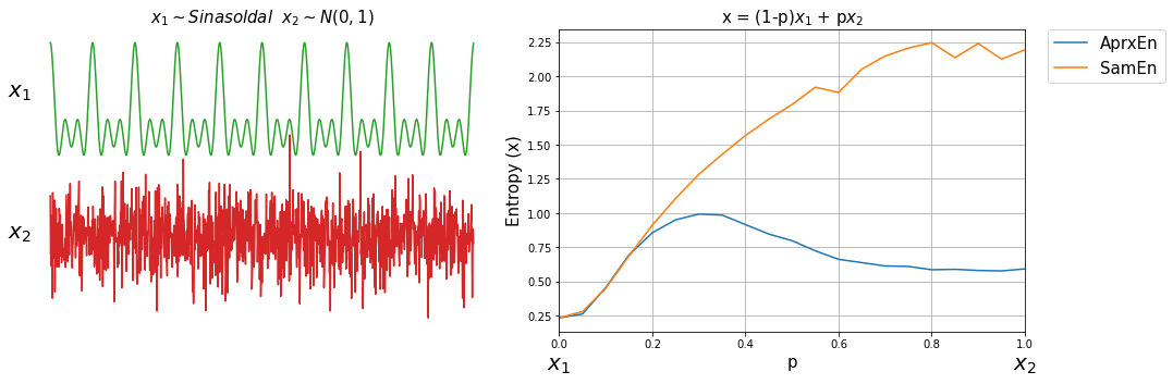
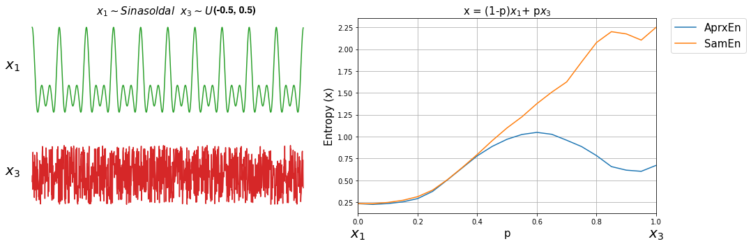
Approximate Entropy Vs Sample Entropy

Sample entropy was proposed as the improved version of Approximate entropy, here we can compare both with a small simulation

First, lets compare the already computed values and time taken by each function

print('  \t Approx Entropy \t Sample Entropy')
print('--'*30)
print(f'x1:\t {Hx1_apx} \t {Hx1_sae}')
print(f'x2:\t {Hx2_apx} \t {Hx2_sae}')
print(f'x3:\t {Hx3_apx} \t {Hx3_sae}')

Approximate and Sample Entropy

x (signal)	Approximate Entropy	Sample Entropy
x1 ~ \(\mathcal{Sin}(10,20,30)\)	0.23429427895105137	0.23462714901066314
x2 ~ \(\mathcal{N}(0,1)\)	0.5921334630488566	2.1931512519485836
x3 ~ \(\mathcal{U}(-0.5, 0.5)\)	0.6720444345470105	2.24992380933707

Compare execution time

import time
tt1 = []
for _ in range(5):
  start = time.process_time()
  sp.entropy_approx(x1,m=3,r=0.2*np.std(x1))
  tt1.append(time.process_time() - start)
  print(time.process_time() - start)


tt2 = []
for _ in range(5):
  start = time.process_time()
  sp.entropy_sample(x1,m=3,r=0.2*np.std(x1))
  tt2.append(time.process_time() - start)
  print(time.process_time() - start)


print(f'Approx Entropy:\t {np.mean(tt1)} \t {np.std(tt1)}')
print(f'Sample Entropy:\t {np.mean(tt2)} \t {np.std(tt2)}')

Approximate and Sample Entropy : Time

Entropy fun	mean	sd
Approximate Entropy	3.11875	0.06139
Sample Entropy	0.1625	0.0159

Now, lets compute both entropy values by varies a degree of noise in a signal. This can be done by using a linear combination of x1 and x2, or x1 and x3.

\[x(t) = px1(t) + (1-p)x2(t)\]

\[x(t) = px1(t) + (1-p)x3(t)\]

ApSmEn1 = []
ApSmEn2 = []
SD = []
for i,p in enumerate(np.arange(0,1+0.04,0.05)):
 sp.utils.ProgBar(i,22)

 x41 = x1*(1-p) + p*x2
 aprEn = sp.entropy_approx(x41,m=3,r=0.2*np.std(x41))
 smEn  = sp.entropy_sample(x41,m=3,r=0.2*np.std(x41))
 ApSmEn1.append([p,aprEn,smEn])


 x42 = x1*(1-p) + p*x3
 aprEn = sp.entropy_approx(x42,m=3,r=0.2*np.std(x42))
 smEn  = sp.entropy_sample(x42,m=3,r=0.2*np.std(x42))
 ApSmEn2.append([p,aprEn,smEn])

 SD.append([p,0.2*np.std(x41),0.2*np.std(x42)])

ApSmEn1 = np.array(ApSmEn1)
ApSmEn2 = np.array(ApSmEn2)
SD = np.array(SD)

Singular Value Decomposition Entropy

Hx1_svd = sp.entropy_svd(x1,order=3, delay=1)
Hx2_svd = sp.entropy_svd(x2,order=3, delay=1)
Hx3_svd = sp.entropy_svd(x3,order=3, delay=1)

print(Hx1_svd, Hx2_svd, Hx3_svd)

(0.49681180617094506, 1.5847351068262792, 1.584635658386532)

Permutation Entropy

Hx1_prm = sp.entropy_permutation(x1,order=3, delay=1)
Hx2_prm = sp.entropy_permutation(x2,order=3, delay=1)
Hx3_prm = sp.entropy_permutation(x3,order=3, delay=1)

print(Hx1_prm, Hx2_prm, Hx3_prm)

(1.3785312756717454, 2.583366627307274, 2.5824960835257484)

SVD and Permutation Entropy

x (signal)	SVD Entropy	Permutation Entropy
x1 ~ \(\mathcal{Sin}(10,20,30)\)	0.49681180617094506	1.3785312756717454
x2 ~ \(\mathcal{N}(0,1)\)	1.5847351068262792	2.583366627307274
x3 ~ \(\mathcal{U}(0,1)\)	1.584635658386532	2.5824960835257484

Dispersion Entropy

For Dispersion Entropy, check the next section

---

Examples with EEG Signal

Single Channel

import numpy as np
import matplotlib.pyplot as plt
import spkit as sp
from spkit.data import load_data
print(sp.__version__)

# load sample of EEG segment
X,ch_names = load_data.eegSample()
t = np.arange(X.shape[0])/128
nC = len(ch_names)


x1 =X[:,0] #'AF3' - Frontal Lobe
x2 =X[:,6] #'O1'  - Occipital Lobe
#Shannan entropy
H_x1= sp.entropy(x1,alpha=1)
H_x2= sp.entropy(x2,alpha=1)

#Rényi entropy
Hr_x1= sp.entropy(x1,alpha=2)
Hr_x2= sp.entropy(x2,alpha=2)

print('Shannan entropy')
print('Entropy of x1: H(x1) =\t ',H_x1)
print('Entropy of x2: H(x2) =\t ',H_x2)
print('-')
print('Rényi entropy')
print('Entropy of x1: H(x1) =\t ',Hr_x1)
print('Entropy of x2: H(x2) =\t ',Hr_x2)
print('-')

Multi-Channels (cross)

#Joint entropy
H_x12= sp.entropy_joint(x1,x2)

#Conditional Entropy
H_x12= sp.entropy_cond(x1,x2)
H_x21= sp.entropy_cond(x2,x1)

#Mutual Information
I_x12 = sp.mutual_Info(x1,x2)

#Cross Entropy
H_x12_cross= sp.entropy_cross(x1,x2)

#Diff Entropy
D_x12= sp.entropy_kld(x1,x2)

print('Joint Entropy H(x1,x2) =\t',H_x12)
print('Mutual Information I(x1,x2) =\t',I_x12)
print('Conditional Entropy of : H(x1|x2) =\t',H_x12)
print('Conditional Entropy of : H(x2|x1) =\t',H_x21)
print('-')
print('Cross Entropy of : H(x1,x2) =\t',H_x12_cross)
print('Kullback–Leibler divergence : Dkl(x1,x2) =\t',D_x12)


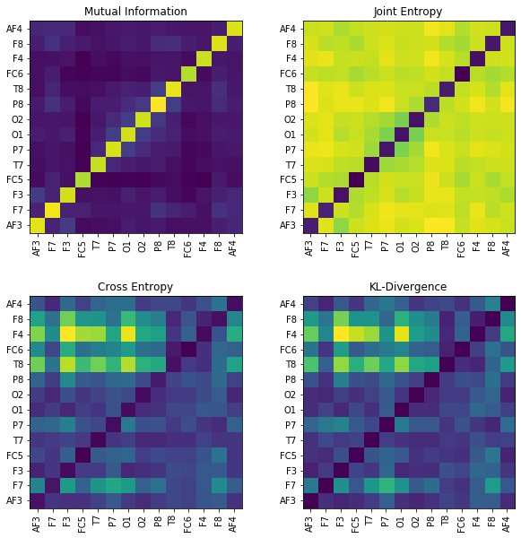
MI = np.zeros([nC,nC])
JE = np.zeros([nC,nC])
CE = np.zeros([nC,nC])
KL = np.zeros([nC,nC])
for i in range(nC):
    x1 = X[:,i]
    for j in range(nC):
        x2 = X[:,j]

        #Mutual Information
        MI[i,j] = sp.mutual_Info(x1,x2)

        #Joint entropy
        JE[i,j]= sp.entropy_joint(x1,x2)

        #Cross Entropy
        CE[i,j]= sp.entropy_cross(x1,x2)

        #Diff Entropy
        KL[i,j]= sp.entropy_kld(x1,x2)



  plt.figure(figsize=(10,10))
  plt.subplot(221)
  plt.imshow(MI,origin='lower')
  plt.yticks(np.arange(nC),ch_names)
  plt.xticks(np.arange(nC),ch_names,rotation=90)
  plt.title('Mutual Information')
  plt.subplot(222)
  plt.imshow(JE,origin='lower')
  plt.yticks(np.arange(nC),ch_names)
  plt.xticks(np.arange(nC),ch_names,rotation=90)
  plt.title('Joint Entropy')
  plt.subplot(223)
  plt.imshow(CE,origin='lower')
  plt.yticks(np.arange(nC),ch_names)
  plt.xticks(np.arange(nC),ch_names,rotation=90)
  plt.title('Cross Entropy')
  plt.subplot(224)
  plt.imshow(KL,origin='lower')
  plt.yticks(np.arange(nC),ch_names)
  plt.xticks(np.arange(nC),ch_names,rotation=90)
  plt.title('KL-Divergence')
  plt.subplots_adjust(hspace=0.3)
  plt.show()

---