Blind Source Separation - ICA Based Artifact Removal
Notebook
View in Jupyter-Notebook
ICA_filtering(X, winsize=128, ICA_method='extended-infomax',
   kur_thr=2, corr_thr=0.8, AF_ch_index=[0, 13],
   F_ch_index=[1, 2, 11, 12],verbose=True)
This algorithm includes following three approaches to removal artifact in EEG
Kurtosis based artifacts - mostly for motion artifacts kur_thr: (default 2) threshold on kurtosis of IC commponents to remove, higher it is, more peaky component is selected
: +ve int value
Correlation Based Index (CBI) for eye movement artifacts For applying CBI method, index of prefrontal (AF - First Layer of electrodes towards frontal lobe) and frontal lobe (F - second layer of electrodes) channels need to be provided. For case of 14-channels Emotiv Epoc * ch_names = [‘AF3’, ‘F7’, ‘F3’, ‘FC5’, ‘T7’, ‘P7’, ‘O1’, ‘O2’, ‘P8’, ‘T8’, ‘FC6’, ‘F4’, ‘F8’, ‘AF4’] * PreProntal Channels =[‘AF3’,’AF4’], * Fronatal Channels = [‘F7’,’F3’,’F4’,’F8’] AF_ch_index =[0,13] : (AF - First Layer of electrodes towards frontal lobe) F_ch_index =[1,2,11,12] : (F - second layer of electrodes) if AF_ch_index or F_ch_index is None, CBI is not applied
Correlation of any independent component with many EEG channels If any indepentdent component is correlated fo corr_thr% (80%) of elecctrodes, is considered to be artifactual – Similar like CBI, except, not comparing fronatal and prefrontal but all corr_thr: (deafult 0.8) threshold to consider correlation, higher the value less IC are removed and vise-versa
: float [0-1], : if None, this is not applied
API
sp.eeg.ICA_filtering(…)
A quick example
import numpy as np
import matplotlib.pyplot as plt
import spkit as sp
from spkit.data import load_data
print(sp.__version__)
X,ch_names = load_data.eegSample()
fs = 128
# high=pass filtering
Xf = sp.filter_X(X,band=[0.5], btype='highpass',fs=fs,verbose=0).T
# ICA Filtering
XR = sp.eeg.ICA_filtering(Xf.copy(),verbose=1,kur_thr=2,corr_thr=0.8,winsize=128)
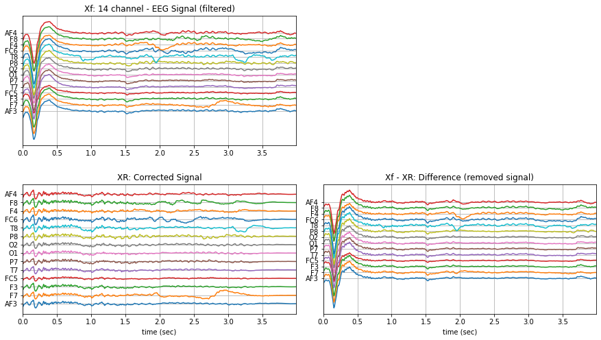
t = np.arange(Xf.shape[0])/fs
plt.figure(figsize=(15,8))
plt.subplot(221)
plt.plot(t,Xf+np.arange(-7,7)*200)
plt.xlim([t[0],t[-1]])
#plt.xlabel('time (sec)')
plt.yticks(np.arange(-7,7)*200,ch_names)
plt.grid()
plt.title('Xf: 14 channel - EEG Signal (filtered)')
plt.subplot(223)
plt.plot(t,XR+np.arange(-7,7)*200)
plt.xlim([t[0],t[-1]])
plt.xlabel('time (sec)')
plt.yticks(np.arange(-7,7)*200,ch_names)
plt.grid()
plt.title('XR: Corrected Signal')
plt.subplot(224)
plt.plot(t,(Xf-XR)+np.arange(-7,7)*200)
plt.xlim([t[0],t[-1]])
plt.xlabel('time (sec)')
plt.yticks(np.arange(-7,7)*200,ch_names)
plt.grid()
plt.title('Xf - XR: Difference (removed signal)')
plt.subplots_adjust(wspace=0.1,hspace=0.3)
plt.show()
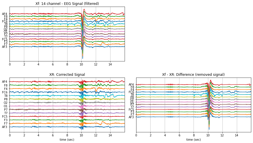
With smaller segment
Xf1 = Xf[128*10:128*14].copy()

XR1 = sp.eeg.ICA_filtering(Xf1.copy(),verbose=1,kur_thr=2,corr_thr=0.8,winsize=128*2)


t = np.arange(Xf1.shape[0])/fs
 plt.figure(figsize=(15,8))
 plt.subplot(221)
 plt.plot(t,Xf1+np.arange(-7,7)*200)
 plt.xlim([t[0],t[-1]])
 #plt.xlabel('time (sec)')
 plt.yticks(np.arange(-7,7)*200,ch_names)
 plt.grid()
 plt.title('Xf: 14 channel - EEG Signal (filtered)')
 plt.subplot(223)
 plt.plot(t,XR1+np.arange(-7,7)*200)
 plt.xlim([t[0],t[-1]])
 plt.xlabel('time (sec)')
 plt.yticks(np.arange(-7,7)*200,ch_names)
 plt.grid()
 plt.title('XR: Corrected Signal')
 plt.subplot(224)
 plt.plot(t,(Xf1-XR1)+np.arange(-7,7)*200)
 plt.xlim([t[0],t[-1]])
 plt.xlabel('time (sec)')
 plt.yticks(np.arange(-7,7)*200,ch_names)
 plt.grid()
 plt.title('Xf - XR: Difference (removed signal)')
 plt.subplots_adjust(wspace=0.1,hspace=0.3)
 plt.show()