Examples

Information Theory - Entropy

View in Jupyter-Notebook

import numpy as np
import matplotlib.pyplot as plt
import spkit as sp

x = np.random.rand(10000)
y = np.random.randn(10000)

#Shannan entropy
H_x= sp.entropy(x,alpha=1)
H_y= sp.entropy(y,alpha=1)

#Rényi entropy
Hr_x= sp.entropy(x,alpha=2)
Hr_y= sp.entropy(y,alpha=2)

H_xy= sp.entropy_joint(x,y)

H_x1y= sp.entropy_cond(x,y)
H_y1x= sp.entropy_cond(y,x)

I_xy = sp.mutual_Info(x,y)

H_xy_cross= sp.entropy_cross(x,y)

D_xy= sp.entropy_kld(x,y)


print('Shannan entropy')
print('Entropy of x: H(x) = ',H_x)
print('Entropy of y: H(y) = ',H_y)
print('-')
print('Rényi entropy')
print('Entropy of x: H(x) = ',Hr_x)
print('Entropy of y: H(y) = ',Hr_y)
print('-')
print('Mutual Information I(x,y) = ',I_xy)
print('Joint Entropy H(x,y) = ',H_xy)
print('Conditional Entropy of : H(x|y) = ',H_x1y)
print('Conditional Entropy of : H(y|x) = ',H_y1x)
print('-')
print('Cross Entropy of : H(x,y) = :',H_xy_cross)
print('Kullback–Leibler divergence : Dkl(x,y) = :',D_xy)

plt.figure(figsize=(12,5))
plt.subplot(121)
sp.HistPlot(x,show=False)

plt.subplot(122)
sp.HistPlot(y,show=False)
plt.show()

Independent Component Analysis - ICA

View in Jupyter-Notebook

from spkit import ICA
from spkit.data import load_data
X,ch_names = load_data.eegSample()

x = X[128*10:128*12,:]
t = np.arange(x.shape[0])/128.0

ica = ICA(n_components=14,method='fastica')
ica.fit(x.T)
s1 = ica.transform(x.T)

ica = ICA(n_components=14,method='infomax')
ica.fit(x.T)
s2 = ica.transform(x.T)

ica = ICA(n_components=14,method='picard')
ica.fit(x.T)
s3 = ica.transform(x.T)

ica = ICA(n_components=14,method='extended-infomax')
ica.fit(x.T)
s4 = ica.transform(x.T)

Machine Learning

Logistic Regression

View more examples in Notebooks

Binary Class

import numpy as np
import matplotlib.pyplot as plt

import spkit
print(spkit.__version__)
0.0.9

from spkit.ml import LogisticRegression

# Generate data
N = 300
np.random.seed(1)
X = np.random.randn(N,2)
y = np.random.randint(0,2,N)
y.sort()

X[y==0,:]+=2 # just creating classes a little far
print(X.shape, y.shape)
plt.plot(X[y==0,0],X[y==0,1],'.b')
plt.plot(X[y==1,0],X[y==1,1],'.r')
plt.show()


clf = LogisticRegression(alpha=0.1)
print(clf)
clf.fit(X,y,max_itr=1000)
yp  = clf.predict(X)
ypr = clf.predict_proba(X)
print('Accuracy : ',np.mean(yp==y))
print('Loss     : ',clf.Loss(y,ypr))

plt.figure(figsize=(12,7))
ax1 = plt.subplot(221)
clf.plot_Lcurve(ax=ax1)
ax2 = plt.subplot(222)
clf.plot_boundries(X,y,ax=ax2)

ax3 = plt.subplot(223)
clf.plot_weights(ax=ax3)
ax4 = plt.subplot(224)
clf.plot_weights2(ax=ax4,grid=False)

Multi Class - with polynomial features

N =300
X = np.random.randn(N,2)
y = np.random.randint(0,3,N)
y.sort()

X[y==0,1]+=3
X[y==2,0]-=3
print(X.shape, y.shape)

plt.plot(X[y==0,0],X[y==0,1],'.b')
plt.plot(X[y==1,0],X[y==1,1],'.r')
plt.plot(X[y==2,0],X[y==2,1],'.g')
plt.show()

clf = LogisticRegression(alpha=0.1,polyfit=True,degree=3,lambd=0,FeatureNormalize=True)
clf.fit(X,y,max_itr=1000)
yp  = clf.predict(X)
ypr = clf.predict_proba(X)
print(clf)
print('')
print('Accuracy : ',np.mean(yp==y))
print('Loss     : ',clf.Loss(clf.oneHot(y),ypr))


plt.figure(figsize=(15,7))
ax1 = plt.subplot(221)
clf.plot_Lcurve(ax=ax1)
ax2 = plt.subplot(222)
clf.plot_boundries(X,y,ax=ax2)

ax3 = plt.subplot(223)
clf.plot_weights(ax=ax3)
ax4 = plt.subplot(224)
clf.plot_weights2(ax=ax4,grid=True)

Naive Bayes

View more examples in Notebooks

import numpy as np
import matplotlib.pyplot as plt

#for dataset and splitting
from sklearn import datasets
from sklearn.model_selection import train_test_split


from spkit.ml import NaiveBayes

#Data
data = datasets.load_iris()
X = data.data
y = data.target

Xt,Xs,yt,ys = train_test_split(X,y,test_size=0.3)

print('Data Shape::',Xt.shape,yt.shape,Xs.shape,ys.shape)

#Fitting
clf = NaiveBayes()
clf.fit(Xt,yt)

#Prediction
ytp = clf.predict(Xt)
ysp = clf.predict(Xs)

print('Training Accuracy : ',np.mean(ytp==yt))
print('Testing  Accuracy : ',np.mean(ysp==ys))


#Probabilities
ytpr = clf.predict_prob(Xt)
yspr = clf.predict_prob(Xs)
print('\nProbability')
print(ytpr[0])

#parameters
print('\nParameters')
print(clf.parameters)


#Visualising
clf.set_class_labels(data['target_names'])
clf.set_feature_names(data['feature_names'])


fig = plt.figure(figsize=(10,8))
clf.VizPx()

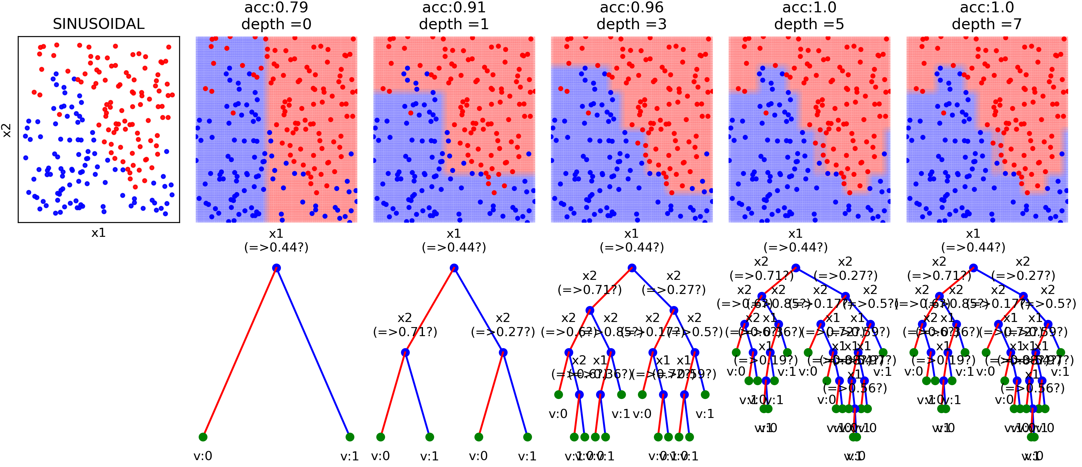
Decision Trees

View more examples in Notebooks

Or just execute all the examples online, without installing anything

One example file is

import numpy as np
import matplotlib.pyplot as plt

# Data and Split
from sklearn.model_selection import train_test_split
from sklearn.datasets import load_diabetes

from spkit.ml import ClassificationTree


data = load_diabetes()
X = data.data
y = 1*(data.target>np.mean(data.target))

feature_names = data.feature_names
print(X.shape, y.shape)
Xt,Xs,yt,ys = train_test_split(X,y,test_size =0.3)
print(Xt.shape, Xs.shape,yt.shape, ys.shape)


clf = ClassificationTree(max_depth=7)
clf.fit(Xt,yt,feature_names=feature_names)
ytp = clf.predict(Xt)
ysp = clf.predict(Xs)

ytpr = clf.predict_proba(Xt)[:,1]
yspr = clf.predict_proba(Xs)[:,1]

print('Depth of trained Tree ', clf.getTreeDepth())
print('Accuracy')
print('- Training : ',np.mean(ytp==yt))
print('- Testing  : ',np.mean(ysp==ys))
print('Logloss')
Trloss = -np.mean(yt*np.log(ytpr+1e-10)+(1-yt)*np.log(1-ytpr+1e-10))
Tsloss = -np.mean(ys*np.log(yspr+1e-10)+(1-ys)*np.log(1-yspr+1e-10))
print('- Training : ',Trloss)
print('- Testing  : ',Tsloss)

# Plot Tree
plt.figure(figsize=(15,12))
clf.plotTree()

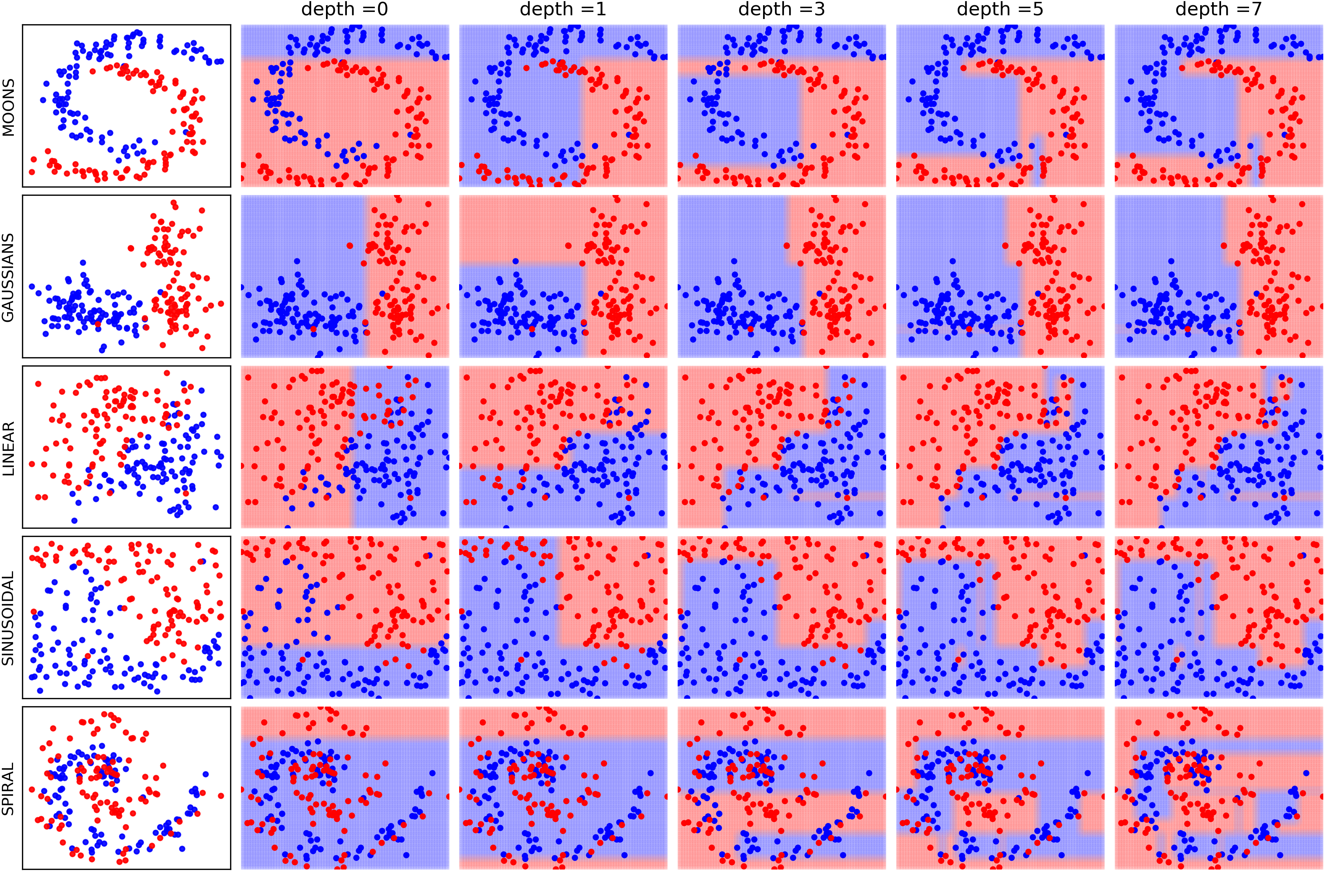
Plottng tree while training

Linear Feedback Shift Register

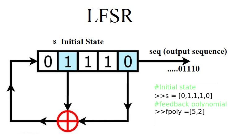
Example: 5 bit LFSR with x^5 + x^2 + 1

import numpy as np
from spkit.pylfsr import LFSR

L = LFSR()
L.info()
L.next()
L.runKCycle(10)
L.runFullCycle()
L.info()
tempseq = L.runKCycle(10000)    # generate 10000 bits from current state

Check out more examples of LFSR**